Main navigation
User account menu
Language
From the new available dataset in GFW on tree cover change between 2000 and 2020, here we are displaying the net change in tree cover by percent for country.The net change in tree cover corresponds to the area of gross gain minus the area of gross loss to show the overall change (negative or positive). The attribute table provides also statistics on net change in tree cover such stable forest or disturbed forest(in hectars).
This dataset is accessed through Global Forest Watch on 04/10/2022. www.globalforestwatch.org.
Potapov, P., Hansen, M.C., Pickens, A., Hernandez-Serna, A., Tyukavina, A., Turubanova, S., Zalles, V., Li, X., Khan, A., Stolle, F., Harris, N., Song, X-P., Baggett, A., Kommareddy, I., and Kommareddy, A. 2022. The Global 2000-2020 Land Cover and Land Use Change Dataset Derived From the Landsat Archive: First Results. Frontiers in Remote Sensing, 13, April 2022. https://doi.org/10.3389/frsen.2022.856903; summarized by administrative area at WRI
This dataset provides projections of global rainfall erosivity changes, a critical metric representing the erosive force of rainfall that drives worldwide soil and nutrient loss. These maps serve as essential inputs for global and regional soil erosion assessment models. The collection details the geographical distribution of projected erosivity changes across two primary periods: 2010–2050 and 2050–2070. To account for different climate trajectories, the dataset includes models for three distinct Representative Concentration Pathway (RCP) scenarios for both timeframes: RCP 2.6 (stringent mitigation), RCP 4.5 (intermediate emissions), and RCP 8.5 (high emissions). By combining these temporal and climatic variables, users can evaluate and compare potential future soil erosion risks under varying degrees of global climate change.
Malaria, a life-threatening disease transmitted by mosquitoes, affects millions of people worldwide. Treatment and prevention efforts such as insecticide-treated mosquito nets and rapid diagnostic tests significantly decreased the number of malaria cases in Africa. This layer displays the change in malaria rates (%) from 2000 to 2015 among children in Sub-Saharan Africa.
Park managers in many countries across Africa need to monitor and understand their parks features and overall health. They can rely on the highly detailed land cover information offered by the Copernicus Hot Spot Land Cover Change Explorer for specific areas of interest –or hot spots. These areas were selected for their importance in biodiversity preservation (Protected Areas, Key Landscapes for Conservation...). For each land cover class (Natural vegetation, Wetlands, urbane areas, etc.), this layer shows which portions of the areas changed to another class over the period (2000-2019). For a more detailed analysis, compare the layer with the present landcover or refer to the online Explorer. The allows to monitor land cover and land cover change in high detail and make informed decisions based on spatial data.
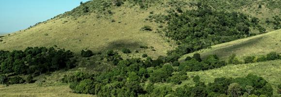
The EC JRC global map of forest cover provides a spatially explicit representation of forest presence and absence for the year 2020 at 10m spatial resolution.
The year 2020 corresponds to the cut-off date of the Regulation from the European Union "on the making available on the Union market and the export from the Union of certain commodities and products associated with deforestation and forest degradation" (EUDR, Regulation (EU) 2023/1115). In the context of the EUDR, the global forest cover map can be used as a non-mandatory, non-exclusive, and not legally binding source of information. Further information about the map and its use can be found on the EU Observatory on Deforestation and Forest Degradation (EUFO) in the section on Frequently Asked Questions.
Forest means land spanning more than 0.5 hectares with trees higher than 5 meters and a canopy cover of more than 10%, or trees able to reach those thresholds in situ, excluding land that is predominantly under agricultural or urban land use. Agricultural use means the use of land for the purpose of agriculture, including for agricultural plantations (i.e. tree stands in agricultural production systems such as fruit tree plantations, oil palm plantations, olive orchards and agroforestry systems) and set- aside agricultural areas, and for rearing livestock. All plantations of relevant commodities other than wood, that is cattle, cocoa, coffee, oil palm, rubber, soya, are excluded from the forest definition.
The global map of forest cover was created by combining available global datasets (wall-to-wall or global in their scope) on tree cover, tree height, land cover and land use into a single harmonized globally-consistent representation of where forests existed in 2020.
The workflow consisted in first mapping the global maximum extent of tree cover circa the year 2020 from the combination of ESA World Cover 2020 and 2021, WRI Tropical Tree Cover 2020, UMD Global land cover and land use 2019, Global Mangrove Watch 2020, and JRC Tropical Moist Forest 2020 datasets. In the second step, a series of overlays and decision rules were applied to reduce this maximum extent of tree cover and align it with the Forest definition using datasets covering cropland and commodity expansion (ESA World Cereal, UMD Global land cover and land use 2019, UMD Global Cropland Expansion, High-resolution global map of smallholder and industrial oil palm plantations, and WRI Spatial Database of Planted Trees), land use change (UMD global forest cover loss, JRC Tropical Moist Forest, IIASA Global Forest Management), built-up (JRC Global Human Settlement), and water (JRC Global Surface Water).
The detailed mapping approach will be described in a separate technical report expected to be released by March 2024. The accuracy of this map has not been yet assessed but will be reported as soon as available.
Please also refer to the list of known issues and to the JRC Data Catalogue entry.
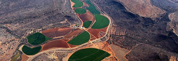
Land cover is defined as the physical material at the surface of the earth, usually documented via the interpretation of earth observations. Common land cover types include trees, grass, bare ground, built up areas, water, etc. How well are different ecosystem types (as indicated by land cover) preserved and how strong are anthropogenic changes affecting their distribution in a given area? Human pressures are constantly increasing and it is important to monitor the consequences of the associated changes on the environment. This map shows the changes in land cover between 1995 and 2015.

Net official development assistance (ODA) is government aid designed to promote the economic development and welfare of developing countries. Aid may be provided bilaterally, from donor to recipient, or channelled through a multilateral development agency such as the United Nations or the World Bank. Net official aid (OA) refers to aid flows from official donors to more advanced (developing) countries and territories. Official aid is provided under terms and conditions similar to those for ODA. This map shows the aggregated figure (sum of ODA and OA) for African countries. Data are in current U.S. dollars.
Forests worldwide are in a state of flux, with accelerating losses in some regions and gains in others. Given the recognized importance of forest ecosystem services, quantification of global forest extent and change is needed. This map displays the tree cover in the year 2000. Tree cover is defined as canopy closure for all vegetation taller than 5m in height and is expressed as a percentage per output grid cell, in the range 0–100.
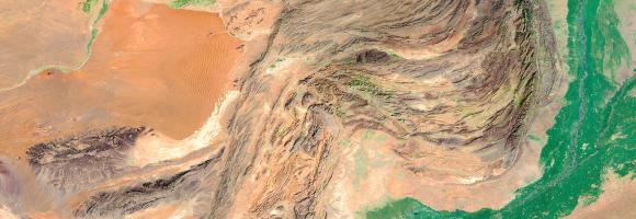
Some extraordinary changes have occurred across the globe over the past decades regarding human habitation. Globally, between 1975 and 2015 built-up areas increased by approximately 250 %, while population increased by a factor of 1.8. The most considerable changes occurred in Africa where it has nearly quadrupled. The extent of built-up area poses a number of challenges to global sustainable development. As urban clusters expand, productive land and soil is sealed, and natural ecosystems are replaced by land use to support urban centres. This layer highlights the areas of concern for built-up related issues derived from the convergence of global evidence of human-environment interactions that can have land degradation consequences.
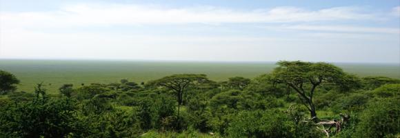
The data provided here are the result of a time-series analysis of carbon density change (in Mg/ha) between 2003-2014 spanning tropical America, Africa, and Asia (23.45 N lat.-23.45 S lat.). The original data is provided as two separate rasters representing (1) carbon density net gain and (2) carbon density net loss within each ~463 x 463 metre pixel, with only pixels exhibiting statistical significance at the 95% level being reported. The data here was re-projected from the its original MODIS sinusoidal projection to WGS84.
During the last twenty years (2000-2020) the intact forest landscapes extent within African, Caribbean and Pacific countries, decreased by 16% (237275km2).
However the protection of IFLs increased in the last two decades. Since 2000, around 100 conserved and protected areas were created in intact forests areas in ACP countries, increasing the percentage of IFL protected from 11% in 2000 to 26% in 2020.. Ethiopia has proposed six protected areas that will cover the total extent of IFL in the country. Republic of Congo increased IFL protection from 15,78% in 2000 to 67,07% in 2020.
| Country | Percentage protected in 2000 | Percentage protected in 2013 | Percentage protected in 2016 | Percentage protected in 2020 |
| Angola | 0.00 | 0.00 | 0 | 0.00 |
| Belize | 90.63 | 92.14 | 91.44447 | 91.99 |
| Cote d'Ivoire | 45.76 | 68.62 | 70.72509 | 82.37 |
| Cameroon | 98.89 | 99.96 | 99.96414 | 99.97 |
| Central African Republic | 14.20 | 39.23 | 47.47338 | 60.00 |
| Congo | 12.65 | 19.72 | 21.21028 | 22.03 |
| Cuba | 15.78 | 59.62 | 63.48035 | 67.07 |
| Democratic Republic of the Congo | 0.00 | 100.00 | 100 | 100.00 |
| Dominican Republic | 0.00 | 98.05 | 98.04902 | 98.05 |
| Equatorial Guinea | 1.07 | 0.00 | 0 | 0.00 |
| Ethiopia | 5.23 | 27.32 | 28.38109 | 29.74 |
| Gabon | 36.57 | 66.72 | 72.62826 | 73.61 |
| Guyana | 2.89 | 12.50 | 12.99736 | 13.25 |
| Liberia | 29.30 | 43.19 | 43.42341 | 54.63 |
| Madagascar | 34.84 | 39.28 | 37.74979 | 91.96 |
| Nigeria | 88.66 | 89.20 | 89.64465 | 91.54 |
| Papua New Guinea | 2.36 | 3.50 | 3.627328 | 4.61 |
| Samoa | 0.00 | 0.00 | 0 | 2.29 |
| Solomon Islands | 11.64 | 16.82 | 17.09852 | 18.69 |
| Suriname | 83.56 | 86.31 | 85.87311 | 95.55 |
| Uganda | 96.84 | 97.64 | 97.85507 | 98.25 |
| United Republic of Tanzania | 2.02 | 1.91 | 1.906882 | 1.92 |
| Vanuatu | 0.00 | 14.54 | 14.54262 | 14.48 |
Analysis performed by Simona Lippi
Reference:
Potapov, P., Hansen, M. C., Laestadius L., Turubanova S., Yaroshenko A., Thies C., Smith W.,
Zhuravleva I., Komarova A., Minnemeyer S., Esipova E. “The last frontiers of wilderness: Tracking loss of
intact forest landscapes from 2000 to 2013” Science Advances, 2017; 3:e1600821
''Intact Forest Landscapes (IFLs) are defined as those with an unfragmented area of at least 500 km2 and which are minimally influenced by human economic activity''.(Thies et al. 2011) IFLs are critical for stabilizing terrestrial carbon storage, harboring biodiversity, regulating hydrological regimes, and providing other ecosystem functions. Researchers, firstly, created a global IFL map using existing fine-scale maps and
a global coverage of high spatial resolution satellite imagery (Potapov et al. 2008). Moreover they assessed the distribution and dynamics of IFLs within the extent of present-day forest ecosystems tracking loss of intact forest landscapes from 2000 to 2020. In this layer we show the reduction of the IFL extent for African, Caribbean and Pacific (ACP)countries that decreased by 16,6% since the year 2000. Countries that experienced the largest reduction in intact forest landscape area over the past two decades are Solomon Islands with 66,3 %, Central African Republic with 57% and Equatorial Guinea with 50,4%. Democratic Republic of the Congo still has the highest proportion of intactness of ACP countries with 59,7Mha. IFL in Democratic Republic of the Congo has an extent of 64,3Mha as the 27,7% of its forest cover.
| Country | IFL Area in 2000 (sqkm) | IFL Area in 2020 (sqkm) | Percentage of IFL reduction |
| Angola | 2913.32 | 1752.85 | 39.83 |
| Belize | 4275.28 | 3598.44 | 15.83 |
| Cote d'Ivoire | 4558.78 | 3760.48 | 17.51 |
| Cameroon | 52752.96 | 31968.77 | 39.40 |
| Central African Republic | 8695.96 | 3727.14 | 57.14 |
| Congo | 138699.28 | 100215.44 | 27.75 |
| Cuba | 544.02 | 544.02 | 0.00 |
| Democratic Republic of the Congo | 643864.37 | 597275.75 | 7.24 |
| Dominican Republic | 795.21 | 564.89 | 28.96 |
| Equatorial Guinea | 4249.57 | 2104.83 | 50.47 |
| Ethiopia | 3671.63 | 3233.76 | 11.93 |
| Gabon | 108838.30 | 76291.78 | 29.90 |
| Guyana | 144296.97 | 117327.95 | 18.69 |
| Liberia | 4748.74 | 2880.65 | 39.34 |
| Madagascar | 17240.16 | 10799.08 | 37.36 |
| Nigeria | 2959.07 | 2416.10 | 18.35 |
| Papua New Guinea | 159523.52 | 127121.71 | 20.31 |
| Samoa | 650.86 | 643.16 | 1.18 |
| Solomon Islands | 7820.33 | 2630.05 | 66.37 |
| Suriname | 107282.59 | 92574.26 | 13.71 |
| Uganda | 984.66 | 962.06 | 2.30 |
| United Republic of Tanzania | 4081.92 | 3796.32 | 7.00 |
| Vanuatu | 706.13 | 688.33 | 2.52 |
Côte d'Ivoire and Ghana are the main largest producers of cocoa in the world. However, the cultivation of this crop has led to the loss of vast tracts of forest areas in both countries. Efficient and accurate methods for remotely identifying cocoa farms are essential for the implementation of sustainable cocoa practices and the periodic and effective monitoring of forests. This map, generated using Random Forest image classification, shows the 2019 distribution of cocoa farms in both countries. The estimated area for cocoa is 4.8Mha for Cote d'Ivoire and 2.3Mha for Ghana.
An intact forest landscape (IFL) is a seamless mosaic of forest and naturally treeless ecosystems with no remotely detected signs of human activity and a minimum area of 500 km2. (Potapov et al.2017) Intact forests are complex and diverse ecosystems that if lost, are irreplaceable. Research shows that designating intact forest landscapes as protected areas has proven effective at limiting their fragmentation. Since 2000, around 100 conserved and protected areas were created in intact forests areas in ACP countries, increasing the percentage of IFL protected from 11% in 2000 to 26% in 2020.
Differences in countries in terms of IFL area reduction: Cuba has not experienced any reduction in IFLs and nowadays its intact forests are fully protected by PAs (544sqkm). At the contrary Angola still not has any kind of protection for its IFLs and experienced a reduction of 39,83% of its IFL (1160 sqkm) in country.The reduction of IFL area in ACP countries was higher outside PAs (19%) than within PAs (5%).Madagascar is the country where the reduction of IFL areas was very high inside protected areas (2420 sqkm). The IFL loss inside PAs has been more than 40% between 2000 and 2020. Central African Republic experienced 23% of reduction inside PAs (938,13 sqkm). This layer shows the percentage of IFLs protected by country
| Country | IFL protected 2020 (sqkm) | IFL unprotected 2020 (sqkm) | Percentage of IFL protected 2020 | Percentage of IFL unprotected 2020 |
| Angola | 0.00 | 1752.85 | 0.00 | 100.00 |
| Belize | 3310.17 | 288.36 | 91.99 | 8.01 |
| Cameroon | 19181.16 | 12787.52 | 60.00 | 40.00 |
| Central African Republic | 3070.21 | 656.90 | 82.37 | 17.62 |
| Congo | 67218.88 | 32997.23 | 67.07 | 32.93 |
| Cote d'Ivoire | 3759.21 | 1.27 | 99.97 | 0.03 |
| Cuba | 544.02 | 0.00 | 100.00 | 0.00 |
| Democratic Republic of the Congo | 131588.22 | 465687.18 | 22.03 | 77.97 |
| Dominican Republic | 553.86 | 11.03 | 98.05 | 1.95 |
| Equatorial Guinea | 1549.39 | 555.44 | 73.61 | 26.39 |
| Ethiopia | 0 | 3233.7 | 0 | 100 |
| Gabon | 22692.90 | 53598.80 | 29.74 | 70.26 |
| Guyana | 15545.93 | 101781.93 | 13.25 | 86.75 |
| Liberia | 1573.69 | 1306.95 | 54.63 | 45.37 |
| Madagascar | 9931.34 | 867.74 | 91.96 | 8.04 |
| Nigeria | 2211.75 | 204.39 | 91.54 | 8.46 |
| Papua New Guinea | 5863.48 | 121258.17 | 4.61 | 95.39 |
| Samoa | 93.13 | 550.03 | 14.48 | 85.52 |
| Solomon Islands | 60.11 | 2569.93 | 2.29 | 97.71 |
| Suriname | 17304.85 | 75269.36 | 18.69 | 81.31 |
| Uganda | 945.21 | 16.84 | 98.25 | 1.75 |
| United Republic of Tanzania | 3627.46 | 168.85 | 95.55 | 4.45 |
| Vanuatu | 13.24 | 675.08 | 1.92 | 98.08 |
Analysis performed by Simona Lippi
At any given place on Earth, complex human-environment interactions are at play. They include differing rates and magnitudes of drivers (e.g. overgrazing, climate change, agricultural practices) and differing consequences in land degradation (e.g. soil erosion, changes in productivity, loss of biodiversity). The occurrence of multiple global change issues at a location suggests a potential for land degradation, at least in some form. This layer depicts where global change issues relevant to land degradation coincide at a global scale. It helps identifying local or regional areas of concern where land degradation processes may be underway.
Whether you’re monitoring crops, modelling green energy installations or soil sealing, combatting loss of natural resources or just helping countries meet their Sustainable Development Goals, chances are high that you’ll need an accurate and spatially detailed map on land cover and land use. Earth Observation satellites, like those from EU’s flagship programme Copernicus, are key to providing such maps, at a global scale, with free and open access. Land cover maps represent spatial information on different types (classes) of physical coverage of the Earth's surface, e.g. forests, grasslands, croplands, lakes, wetlands. Dynamic land cover maps include transitions of land cover classes over time and hence captures land cover changes. This dataset shows the land cover for the baseline year 2019 with a discrete classification in 23 classes aligned with UN-FAO's Land Cover Classification System.
Copernicus is the European flagship programme for monitoring the Earth. Data is collected by Earth observation satellites and sensors on the earth’s surface. The Copernicus Land Monitoring Service provides geographical information on land use and land cover at European and global scale. Derived from the Copernicus Hot Spot Land Cover Change Explorer, this layer presents detailed land cover information for specific areas of interest –or hot spots– in Africa. These areas were selected as a priority for mapping because of their importance in biodiversity preservation (Protected Areas, Key Landscapes for Conservation...). Park managers in many countries across Africa rely on this Copernicus product to monitor and understand their parks features and overall health. Mapping habitats, assessing pressure on land, identifying prime locations for species reintroduction or new areas to protect are just a few examples of how these data can be exploited.
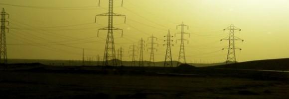
In Sub-Saharan Africa, medium- and low-voltage data are often non-existent, uncompleted, or unavailable. This is a challenge for practitioners working on the electricity access agenda, power sector resilience or climate change adaptation. This layer presents the spatial extent of the existing and planned electricity grid (high, medium, low voltage level) compiled using multiple sources that enumerate elements of the existing transmission and distribution network.
This dataset provides the P50 projections for a geothermal system utilizing a Chiller unit.
Chiller refers to an absorption chiller or heat pump integrated into the geothermal system. It is used to provide cooling (by utilizing the geothermal heat) or to extract additional heat from the return fluid, thereby increasing the system's overall thermal harvest.
P50 is a statistical term used in risk analysis and forecasting. P50 represents the median scenario, meaning there is a 50% probability that the actual outcome will be higher than this value and a 50% probability it will be lower. It serves as the baseline "best estimate."
Metrics DefinitionsCoefficient of Performance (COP) [-]: A measure of efficiency, defined as the ratio of useful heating or cooling provided to the work (energy) required to operate the Chiller. Higher values indicate greater efficiency.
Doublet Net Production [MW]: The actual useful power output (Megawatts) generated by the "doublet" (one production well + one injection well), subtracting any energy used by pumps or auxiliary equipment.
Levelized Cost of Energy (LCOE) [US$ct/kWh]: The average revenue per unit of energy needed to recover the cost of building and operating the plant over its entire life cycle. It essentially represents the break-even price.
Net Present Value (NPV) [million US$]: The current financial value of all future cash flows the project will generate, minus the initial investment costs. A positive NPV generally indicates a profitable project.
Optimized Depth of the Aquifer [m]: The calculated ideal drilling depth (meters) to reach the geothermal reservoir that balances drilling costs with temperature/flow benefits.
Production Flow Rate [m³/h]: The volume of geothermal fluid extracted from the reservoir per hour (cubic meters per hour).
Temperature at Reservoir [°C]: The natural temperature (Celsius) of the geothermal fluid within the subsurface rock formation before it is brought to the surface.
Transmissivity [Dm]: A measure of how easily fluid flows through the porous aquifer. It is the product of hydraulic conductivity and aquifer thickness (often measured in Darcy-meters). High transmissivity means easier extraction.
Well Distance [m]: The physical distance (meters) between the production well (extraction) and the injection well (return). Proper spacing prevents "short-circuiting," where cool injected water lowers the temperature of the production well too quickly.
This dataset provides the P50 projections for a Direct Heat geothermal system.
Direct Heat refers to the use of geothermal energy for applications such as space heating, industrial processes, or agriculture. In the utilized model, it is assumed a minimum production temperature of at least 60°C and a reinjection temperature of 40°C.
P50 is a statistical term used in risk analysis and forecasting. P50 represents the median scenario, meaning there is a 50% probability that the actual outcome will be higher than this value and a 50% probability it will be lower. It serves as the baseline "best estimate."
Metrics DefinitionsCoefficient of Performance (COP) [-]: A measure of efficiency, defined as the ratio of useful heating or cooling provided to the work (energy) required to operate the Chiller. Higher values indicate greater efficiency.
Doublet Net Production [MW]: The actual useful power output (Megawatts) generated by the ""doublet"" (one production well + one injection well), subtracting any energy used by pumps or auxiliary equipment.
Levelized Cost of Energy (LCOE) [US$ct/kWh]: The average revenue per unit of energy needed to recover the cost of building and operating the plant over its entire life cycle. It essentially represents the break-even price.
Net Present Value (NPV) [million US$]: The current financial value of all future cash flows the project will generate, minus the initial investment costs. A positive NPV generally indicates a profitable project.
Optimized Depth of the Aquifer [m]: The calculated ideal drilling depth (meters) to reach the geothermal reservoir that balances drilling costs with temperature/flow benefits.
Production Flow Rate [m³/h]: The volume of geothermal fluid extracted from the reservoir per hour (cubic meters per hour).
Temperature at Reservoir [°C]: The natural temperature (Celsius) of the geothermal fluid within the subsurface rock formation before it is brought to the surface.
Transmissivity [Dm]: A measure of how easily fluid flows through the porous aquifer. It is the product of hydraulic conductivity and aquifer thickness (often measured in Darcy-meters). High transmissivity means easier extraction.
Well Distance [m]: The physical distance (meters) between the production well (extraction) and the injection well (return). Proper spacing prevents ""short-circuiting,"" where cool injected water lowers the temperature of the production well too quickly.
This dataset provides the P50 projections for a Direct Heat with Heat Pump geothermal system.
Direct Heat with Heat Pump refers to a scenario where a geothermal system is integrated with an industrial heat pump to upgrade low-grade heat. This allows for production from geothermal temperatures as low as 40°C, which are then heated by the pump to a delivery temperature of 80°C. The reinjection temperature is set to the production temperature minus 20°C, with a absolute minimum of 15°C.
P50 is a statistical term used in risk analysis and forecasting. P50 represents the median scenario, meaning there is a 50% probability that the actual outcome will be higher than this value and a 50% probability it will be lower. It serves as the baseline ""best estimate.""
Metrics DefinitionsCoefficient of Performance (COP) [-]: A measure of efficiency, defined as the ratio of useful heating or cooling provided to the work (energy) required to operate the Chiller. Higher values indicate greater efficiency.
Doublet Net Production [MW]: The actual useful power output (Megawatts) generated by the ""doublet"" (one production well + one injection well), subtracting any energy used by pumps or auxiliary equipment.
Levelized Cost of Energy (LCOE) [US$ct/kWh]: The average revenue per unit of energy needed to recover the cost of building and operating the plant over its entire life cycle. It essentially represents the break-even price.
Net Present Value (NPV) [million US$]: The current financial value of all future cash flows the project will generate, minus the initial investment costs. A positive NPV generally indicates a profitable project.
Optimized Depth of the Aquifer [m]: The calculated ideal drilling depth (meters) to reach the geothermal reservoir that balances drilling costs with temperature/flow benefits.
Production Flow Rate [m³/h]: The volume of geothermal fluid extracted from the reservoir per hour (cubic meters per hour).
Temperature at Reservoir [°C]: The natural temperature (Celsius) of the geothermal fluid within the subsurface rock formation before it is brought to the surface.
Transmissivity [Dm]: A measure of how easily fluid flows through the porous aquifer. It is the product of hydraulic conductivity and aquifer thickness (often measured in Darcy-meters). High transmissivity means easier extraction.
Well Distance [m]: The physical distance (meters) between the production well (extraction) and the injection well (return). Proper spacing prevents ""short-circuiting,"" where cool injected water lowers the temperature of the production well too quickly.
This dataset provides the P50 projections for an Organic Rankine Cycle (ORC) geothermal power plant.
Organic Rankine Cycle (ORC) refers to a binary power plant configuration where geothermal fluid (brine) is used to heat a secondary organic working fluid. This process allows for efficient electricity generation from medium-to-low temperature resources (typically 90°C to 150°C). The organic fluid vaporizes, drives a turbine, and is then condensed back into a liquid to repeat the cycle. The geothermal brine is reinjected into the reservoir after passing through the heat exchanger.
P50 is a statistical term used in risk analysis and forecasting. P50 represents the median scenario, meaning there is a 50% probability that the actual outcome will be higher than this value and a 50% probability it will be lower. It serves as the baseline ""best estimate.""
Metrics DefinitionsCoefficient of Performance (COP) [-]: A measure of efficiency, defined as the ratio of useful heating or cooling provided to the work (energy) required to operate the Chiller. Higher values indicate greater efficiency.
Doublet Net Production [MW]: The actual useful power output (Megawatts) generated by the ""doublet"" (one production well + one injection well), subtracting any energy used by pumps or auxiliary equipment.
Levelized Cost of Energy (LCOE) [US$ct/kWh]: The average revenue per unit of energy needed to recover the cost of building and operating the plant over its entire life cycle. It essentially represents the break-even price.
Net Present Value (NPV) [million US$]: The current financial value of all future cash flows the project will generate, minus the initial investment costs. A positive NPV generally indicates a profitable project.
Optimized Depth of the Aquifer [m]: The calculated ideal drilling depth (meters) to reach the geothermal reservoir that balances drilling costs with temperature/flow benefits.
Production Flow Rate [m³/h]: The volume of geothermal fluid extracted from the reservoir per hour (cubic meters per hour).
Temperature at Reservoir [°C]: The natural temperature (Celsius) of the geothermal fluid within the subsurface rock formation before it is brought to the surface.
Transmissivity [Dm]: A measure of how easily fluid flows through the porous aquifer. It is the product of hydraulic conductivity and aquifer thickness (often measured in Darcy-meters). High transmissivity means easier extraction.
Well Distance [m]: The physical distance (meters) between the production well (extraction) and the injection well (return). Proper spacing prevents ""short-circuiting,"" where cool injected water lowers the temperature of the production well too quickly.
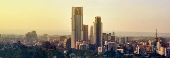
The GHS-BUILT-S spatial raster dataset depicts the distribution of the built-up (BU) surfaces estimates between 1975 and 2030 in 5 year intervals and two functional use components a) the total BU surface and b) the non-residential (NRES) BU surface. The data is made by spatial-temporal interpolation of five observed collections of multiple-sensor, multiple-platform satellite imageries: Landsat (MSS, TM, ETM sensor) data supports the 1975, 1990, 2000, and 2014 epochs, while a Sentinel-2 (S2) image composite (GHS-composite-S2 R2020A) supports the 2018 epoch.
This data represents the total BU surface (square meters) for year 2000 over cells of 1x1 km size.
The GHS-BUILT-S spatial raster dataset depicts the distribution of the built-up (BU) surfaces estimates between 1975 and 2030 in 5 year intervals and two functional use components a) the total BU surface and b) the non-residential (NRES) BU surface. The data is made by spatial-temporal interpolation of five observed collections of multiple-sensor, multiple-platform satellite imageries: Landsat (MSS, TM, ETM sensor) data supports the 1975, 1990, 2000, and 2014 epochs, while a Sentinel-2 (S2) image composite (GHS-composite-S2 R2020A) supports the 2018 epoch.
This data represents the total BU surface estimates (square meters) for year 2000 over cells of 100x100 m size.
The GHS-BUILT-S spatial raster dataset depicts the distribution of the built-up (BU) surfaces estimates between 1975 and 2030 in 5 year intervals and two functional use components a) the total BU surface and b) the non-residential (NRES) BU surface. The data is made by spatial-temporal interpolation of five observed collections of multiple-sensor, multiple-platform satellite imageries: Landsat (MSS, TM, ETM sensor) data supports the 1975, 1990, 2000, and 2014 epochs, while a Sentinel-2 (S2) image composite (GHS-composite-S2 R2020A) supports the 2018 epoch.
This data represents the total BU surface (square meters) for year 2020 over cells of 1x1 km size.
The GHS-BUILT-S spatial raster dataset depicts the distribution of the built-up (BU) surfaces estimates between 1975 and 2030 in 5 year intervals and two functional use components a) the total BU surface and b) the non-residential (NRES) BU surface. The data is made by spatial-temporal interpolation of five observed collections of multiple-sensor, multiple-platform satellite imageries: Landsat (MSS, TM, ETM sensor) data supports the 1975, 1990, 2000, and 2014 epochs, while a Sentinel-2 (S2) image composite (GHS-composite-S2 R2020A) supports the 2018 epoch.
This data represents the total BU surface estimates (square meters) for year 2020 over cells of 100x100 m size.
This data represents the total built-up volume between 1975 and 2030 in 5 year intervals over cells of 1x1 km size.
It derives from the GHS-BUILT-V - R2023A spatial raster dataset, that depicts the distribution of built-up volumes, expressed as number of cubic metres. The data report about the total built-up volume and the built-up volume allocated to dominant non-residential (NRES) uses.
The dataset is part the Global Human Settlement Layer , Global, high-resolution, multi-temporal gridded data on built-up environment (built-up surface, built-up volume, residential vs. non-residential function), resident population, and settlement classification by the UN-recommended methodology “degree of urbanisation”. The complete information about the GHSL main products can be found in the GHSL Data Package 2023 report
This data represents the total built-up volume between 1975 and 2030 in 5 year intervals over cells of 1x1 km size.
It derives from the GHS-BUILT-V - R2023A spatial raster dataset, that depicts the distribution of built-up volumes, expressed as number of cubic metres. The data report about the total built-up volume and the built-up volume allocated to dominant non-residential (NRES) uses.
The dataset is part the Global Human Settlement Layer , Global, high-resolution, multi-temporal gridded data on built-up environment (built-up surface, built-up volume, residential vs. non-residential function), resident population, and settlement classification by the UN-recommended methodology “degree of urbanisation”. The complete information about the GHSL main products can be found in the GHSL Data Package 2023 report
This data represents the distribution of human population between 1975 and 2030 in 5 year intervals over cells of 1x1 km size.
It derives from the GHS-POP - R2023A. Residential population estimates between 1975 and 2020 in 5-year intervals and projections to 2025 and 2030 derived from CIESIN GPWv4.11 were disaggregated from census or administrative units to grid cells, informed by the distribution, volume, and classification of built-up as mapped in the Global Human Settlement Layer (GHSL) global layer per corresponding epoch.
The dataset is part the Global Human Settlement Layer, that provide global, high-resolution, multi-temporal gridded data on built-up environment (built-up surface, built-up volume, residential vs. non-residential function), resident population, and settlement classification by the UN-recommended methodology “degree of urbanisation”. The complete information about the GHSL main products can be found in the GHSL Data Package 2023 report.
This data represents the total built-up volume between 1975 and 2030 in 5 year intervals over cells of 1x1 km size.
It derives from the GHS-BUILT-V - R2023A spatial raster dataset, that depicts the distribution of built-up volumes, expressed as number of cubic metres. The data report about the total built-up volume and the built-up volume allocated to dominant non-residential (NRES) uses.
The dataset is part the Global Human Settlement Layer , Global, high-resolution, multi-temporal gridded data on built-up environment (built-up surface, built-up volume, residential vs. non-residential function), resident population, and settlement classification by the UN-recommended methodology “degree of urbanisation”. The complete information about the GHSL main products can be found in the GHSL Data Package 2023 report
This data represents the distribution of human population between 1975 and 2030 in 5 year intervals over cells of 1x1 km size.
It derives from the GHS-POP - R2023A. Residential population estimates between 1975 and 2020 in 5-year intervals and projections to 2025 and 2030 derived from CIESIN GPWv4.11 were disaggregated from census or administrative units to grid cells, informed by the distribution, volume, and classification of built-up as mapped in the Global Human Settlement Layer (GHSL) global layer per corresponding epoch.
The dataset is part the Global Human Settlement Layer, that provide global, high-resolution, multi-temporal gridded data on built-up environment (built-up surface, built-up volume, residential vs. non-residential function), resident population, and settlement classification by the UN-recommended methodology “degree of urbanisation”. The complete information about the GHSL main products can be found in the GHSL Data Package 2023 report.
This data represents the distribution of human population between 1975 and 2030 in 5 year intervals over cells of 100x100 m size.
It derives from the GHS-POP - R2023A. Residential population estimates between 1975 and 2020 in 5-year intervals and projections to 2025 and 2030 derived from CIESIN GPWv4.11 were disaggregated from census or administrative units to grid cells, informed by the distribution, volume, and classification of built-up as mapped in the Global Human Settlement Layer (GHSL) global layer per corresponding epoch.
The dataset is part the Global Human Settlement Layer, that provide global, high-resolution, multi-temporal gridded data on built-up environment (built-up surface, built-up volume, residential vs. non-residential function), resident population, and settlement classification by the UN-recommended methodology “degree of urbanisation”. The complete information about the GHSL main products can be found in the GHSL Data Package 2023 report.
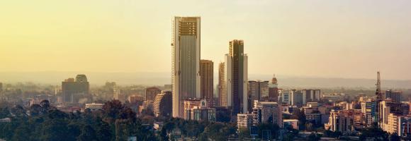
These layers present the application of the Degree of Urbanisation stage I methodology recommended by UN Statistical Commission to the global population grid generated by the JRC in the epochs 1975-2030 (5 years timestep).
They derive from the GHS-SMOD - R2023A.
The layers have been generated by integration of built-up surface extracted from Landsat and Sentinel-2 image data processing (GHS-BUILT-S R2023), and population data derived from the CIESIN GPW v4.11 (GHS-POP R2023).
The dataset is part the Global Human Settlement Layer, that provide global, high-resolution, multi-temporal gridded data on built-up environment (built-up surface, built-up volume, residential vs. non-residential function), resident population, and settlement classification by the UN-recommended methodology “degree of urbanisation”. The complete information about the GHSL main products can be found in the GHSL Data Package 2023 report.
In 2020, a group of researchers carried out analysis to examine the importance of Indigenous Peoples’ lands for preserving Intact Forest Landscapes.(Fa et al.2020)They used geospatial data on the extent of Indigenous Peoples’ lands reported by Garnett et al. (2018), and Geospatial data for IFLs were sourced from the Intact Forest Landscapes website (www.intactforests.org) for the years 2000, 2013, and 2016 (Potapov et al. 2017)In the paper they have shown that the proportion of Indigenous Peoples’ lands mapped as IFLs was considerably higher (10.9%) than the proportion of other lands (defined here as all land outside Indigenous Peoples’ lands) mapped as IFLs (6.8%).
In this map we reported the percentage of Intact Forest Lansdcapes reduction in Indigenous People Lands for the period 2000-2016. IN the table we reported also the percentage of IFLs reduction in other lands. To explore more IFLs conservation strategies for African, Caribbean and Pacific countries you can check BIOPAMA Geonode Layers
Sources:
Fa JE, Watson JE, Leiper I, Potapov P, Evans TD, Burgess ND, Molnár Z, Fernández‐Llamazares Á, Duncan T, Wang S, Austin BJ. Importance of Indigenous Peoples’ lands for the conservation of Intact Forest Landscapes. Frontiers in Ecology and the Environment. 2020 Apr;18(3):135-4

Adult literacy rate is the percentage of people ages 15 and above who can both read and write with understanding a short simple statement about their everyday life. Literacy statistics for most countries cover the population ages 15 and older, but some include younger ages or are confined to age ranges that tend to inflate literacy rates. The youth literacy rate for ages 15-24 reflects recent progress in education. It measures the accumulated outcomes of primary education over the previous 10 years or so by indicating the proportion of the population who have passed through the primary education system and acquired basic literacy and numeracy skills.
The human imprint on the planet has a major impact on the functioning of the Earth system. Because the impact on the environment is closely intertwined with population dynamics, it is important to monitor and include these in the evaluation of land degradation. This layer displays the areas of concern for population change related issues derived from the convergence of global evidence of human-environment interactions that can lead to land degradation. It reflects the dynamics of increasing number of people in a certain area.
This layer is part of the World Altas of Desertification
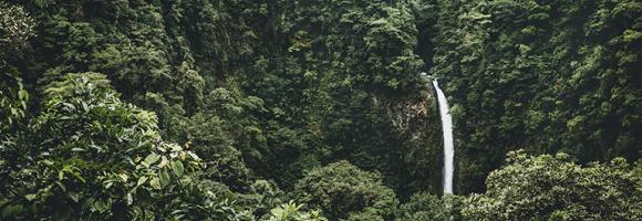
Forests worldwide are in a state of flux, with accelerating losses in some regions and gains in others. Given the recognized importance of forest ecosystem services, quantification of global forest extent and change is needed. This map displays the forest gain during the period 2000–2018. Forest gain is defined as the inverse of loss, or a change from non-forest to forest entirely within the study period. It is expressed as either 1 (gain) or 0 (no gain).
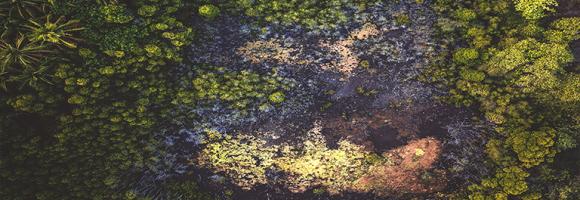
Forests worldwide are in a state of flux, with accelerating losses in some regions and gains in others. Given the recognized importance of forest ecosystem services, quantification of global forest extent and change is needed. This map displays the forest loss during the period 2000–2018, defined as a stand-replacement disturbance, or a change from forest to non-forest state. It is expressed as either 1 (loss - in red) or 0 (no loss).
Forests are the most biologically diverse land ecosystems and are critical for sustaining local and global livelihoods. Deforestation can be considered a type of land degradation when forest ecosystems, with all of their important provisioning, regulating and cultural services, are exchanged for another land use, such as crop agriculture, with a narrow provisioning service focus. Damages to the land resource include the immediate reduction or loss of biomass productivity with a linked loss in habitat, biodiversity, and carbon stock. Clearance of natural forests accelerates soil erosion and the alteration of soil functioning. This layer displays the areas of concern for tree loss issues, derived from the convergence of global evidence of human-environment interactions that can have consequences on land degradation.
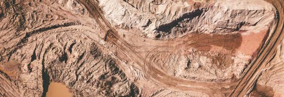
This dataset shows Regional locations and general geologic setting of known deposits of major nonfuel mineral commodities in Africa

This dataset compiles geophysical models detailing the thickness of the Earth's outer layers, ranging from surface sedimentary basins down to the base of the lithosphere. The collection serves a dual purpose: it provides broad, global baseline data for sediment distribution, while also offering high-resolution, integrated regional models specifically focused on the African plate.
Dataset Contents:
I. Global Baselines
II. African Regional Models
These layers are part of the Geothermal Atlas for Africa developed within the LEAP-RE project
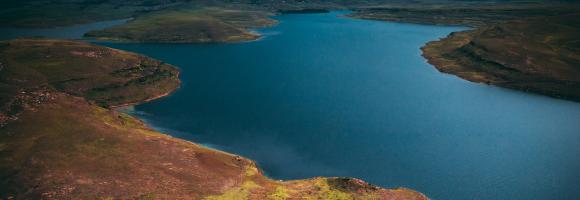
The current version of the GDW database (version 1.0) aims to catalogue all types of anthropogenic instream barriers. While initial mapping efforts prioritize major dams that form reservoirs, as well as run-of-river barriers on larger rivers where more information is readily available, the dataset comprises two distinct but interconnected spatial layers:
<p>This spatial dataset contains the geographic boundaries and ecological evaluations of 45 Key Landscapes for Conservation and Development (KLCDs) across Sub-Saharan Africa. Building on the <a href="https://africa-knowledge-platform.ec.europa.eu/dataset/key-landscapes-c…; Key Landscapes for Conservation (KLCs) </a> identified in the EU report <a href="https://op.europa.eu/sl/publication-detail/-/publication/d76ac7eb-bc4a-…;“Larger than elephants”</a>, the NaturAfrica initiative is rolled out across these key biodiversity and development landscapes.</p>
<p>NaturAfrica's efforts are concentrated on ‘mega-landscapes’—biogeographical regions identified as crucial for both conservation and development. These regions encompass:</p>
<ul>
<li>The forest ecosystems of the Congo Basin;</li>
<li>Landscapes of transhumance pastoralists in North Cameroon, the Central African Republic, and Chad;</li>
<li>Guinean forests of West Africa;</li>
<li>Savannahs in the Sudano-Sahelian zone of West Africa;</li>
<li>Savannahs and watersheds of the East Africa rift;</li>
<li>Transfrontier conservation areas of Southern Africa.</li>
</ul>
<p>The layer was developed to support the prioritization of intervention areas for the second phase of this initiative, which combines conservation with sustainable job creation. It provides a spatially explicit characterization of ecological value across these landscapes, evaluated and attributed based on five core ecological and environmental dimensions:</p>
<ul>
<li><span class="label">Threatened Species Richness:</span> Concentration and diversity of threatened species.</li>
<li><span class="label">Species Endemicity:</span> Presence of endemic species unique to the specific geographic region.</li>
<li><span class="label">Ecosystem Integrity:</span> The integrity of protected and conserved areas, accounting for degrees of human modification and habitat fragmentation.</li>
<li><span class="label">Ecological Connectivity:</span> The degree of connectivity and spatial linkages between protected and conserved areas.</li>
<li><span class="label">Ecosystem Services:</span> Provisioning and regulating services, with a specific focus on carbon storage and water services.</li>
</ul>
<strong>Purpose</strong>
<p>The layer was created to inform the EC Directorate General for International Partnerships (DG INTPA) and policymakers in selecting and prioritizing funding intervention areas based on specific targets (e.g., species conservation, connectivity, or water security) within different biogeographical regions. It serves as a spatial decision-support tool to align with the European Green Deal and the EU Biodiversity Strategy for 2030.</p>
<strong>Geographic Extent</strong>
<ul>
<li><span class="label">Region:</span> Sub-Saharan Africa</li>
<li><span class="label">Coverage:</span> 45 distinct Key Landscapes for Conservation and Development (KLCDs)</li>
</ul>
<strong>Keywords</strong>
<ul>
<li><span class="label">Thematic:</span> Biodiversity Conservation, NaturAfrica, Ecosystem Services, Protected Areas, Habitat Connectivity, Species Endemicity, European Green Deal, Ecosystem Integrity, Transfrontier Conservation, Mega-landscapes.</li>
<li><span class="label">Spatial:</span> Sub-Saharan Africa, Congo Basin, West Africa, East Africa, Southern Africa, Sudano-Sahelian zone.</li>
</ul>
<strong>Lineage / Data Source</strong>
<p>This dataset is derived from the <a href="https://publications.jrc.ec.europa.eu/repository/handle/JRC145021"> technical assessment conducted for the European Commission Knowledge Centre for Biodiversity (KCBD) </a>.</p>
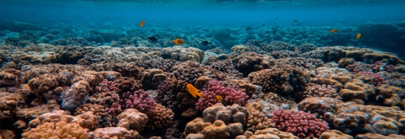
Chlorophyll-a concentrations (Chla) are an indicator of phytoplankton abundance and biomass in open waters. They can be an effective measure of trophic status and are commonly used to measure water quality. This layer compares the Chla value from the last full month with the long-term mean Chla. A positive anomaly (warm colours) means the monthly Chla is higher than the long-term average for that month; a negative anomaly (cool colours) means it is lower than the average.