Main navigation
User account menu
Language

The map is based on Copernicus Global Land Cover data which shows actual land cover (what physically covers land across the globe—forests, grasslands, croplands, lakes, wetlands, built-up area, etc) at 100m x 100m resolution. The land cover data for Africa was overlaid on (high resolution) satellite imagery of Africa, which is then used to determine the land use (by visual interpretation) associated with the various land cover patterns on the Copernicus Global Land Cover map.
Copernicus land cover data offers several advantages: it is of high quality, has a high resolution (100m x 100m), and offers time series satellite imagery. More importantly, the Copernicus Global Land Service is a continuous process and its datasets are updated annually. This means that the Soils4Africa map of agricultural land can be updated every time the land cover data for the new year becomes available (the map is currently based on 2019 data).
The Copernicus dataset already includes the category ‘cropland,’ which by definition is part of agricultural land. The Soils4Africa map broadens the scope of that dataset by infering information on agricultural use and including other kinds of agricultural land use such as grazing pastures and plantations.
When land is mapped as other than ‘cropland'-- like ‘shrubland’ for example-- it is more difficult to interpret and determine whether it is under agricultural use. The Copernicus dataset includes information about ‘fractional cover’-- or the percentage of a particular pixel under a particular kind of land cover (for example, 30% of a 100m x 100m pixel could be forest and 20% could be shrubland). The Soils4Africa map takes into account how fractional cover varies over an area to establish rules for interpreting its land cover data to determine whether it is under agricultural use and for what purpose. These rules were validated by comparing it with ground level information on land use (or land use pattern) for specific areas drawn from the interpretation of satellite imagery from Google Earth.
For example, ground-level observation shows that forest cover upwards of 30% in a given area when matched by shrubland cover of over 30%, is characterized by woody vegetation with a smooth canopy. Therefore, such area is more likely to be under plantations rather than natural forest. Thus, such an area should be counted as agricultural land, even if less than 15% of it is under crops.
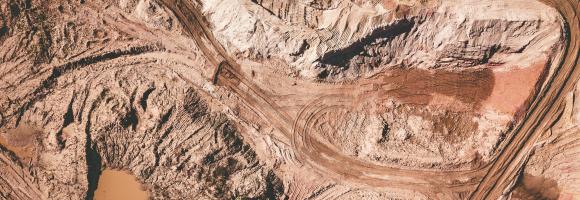
This dataset shows Regional locations and general geologic setting of known deposits of major nonfuel mineral commodities in Africa

The Africa Topographic Potisiont layer classifies the African landscape (including Madagascar, Comoros Islands, and other coastal Islands near continenal Africa) into uplands and lowlands/depressions at a 100m resolution. Published by the USGS in 2009, this dataset was created for the Africa Terrestrial Ecosystems mapping project. The classification is derived from the Compound Topographic Index (CTI) , which integrates slope (from SRTM elevation data) and flow accumulation (from HydroSHEDS data) to model potential water flow.

Map showing the average continental surface temperature of the year 2022. This map was created by interpolating raw monthly satellite data to fill holes in the grids and subsequently adding and averaging the monthly surface temperatures of the year 2022. The data is clipped to only show the African continental region. The raw data is collected during the daytime by the Moderate Resolution Imaging Spectroradiometer (MODIS), an instrument on NASA's Terra and Aqua satellites. Please note that the type of "surface" MODIS measures varies as a function of location. In some places, the measurement represents the skin temperature of the bare land surface. In other places, the temperature represents the skin temperature of whatever is on the land-including snow and ice, or the leafy canopy of forests and crop fields, or human-made structures such as pavement and building rooftops.
Values are expressed in °C.
This dataset is part of the LEAP-RE project collection. For more information visit https://www.leap-re.eu/
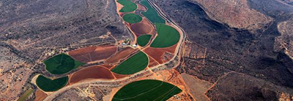
Whether you’re monitoring crops, modelling green energy installations or soil sealing, combatting loss of natural resources or just helping countries meet their Sustainable Development Goals, chances are high that you’ll need an accurate and spatially detailed map on land cover and land use. Earth Observation satellites, like those from EU’s flagship programme Copernicus, are key to providing such maps, at a global scale, with free and open access. Land cover maps represent spatial information on different types (classes) of physical coverage of the Earth's surface, e.g. forests, grasslands, croplands, lakes, wetlands. Dynamic land cover maps include transitions of land cover classes over time and hence captures land cover changes. This dataset shows the land cover for the baseline year 2019 with a discrete classification in 23 classes aligned with UN-FAO's Land Cover Classification System.
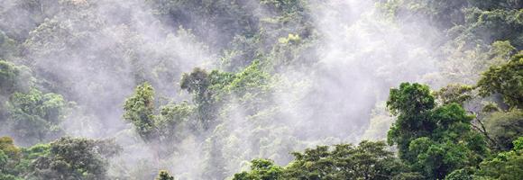
Copernicus is the European flagship programme for monitoring the Earth. Data is collected by Earth observation satellites and sensors on the earth’s surface. The Copernicus Land Monitoring Service provides geographical information on land use and land cover at European and global scale. Derived from the Copernicus Hot Spot Land Cover Change Explorer, this layer presents detailed land cover information for specific areas of interest –or hot spots– in Africa. These areas were selected as a priority for mapping because of their importance in biodiversity preservation (Protected Areas, Key Landscapes for Conservation...). Park managers in many countries across Africa rely on this Copernicus product to monitor and understand their parks features and overall health. Mapping habitats, assessing pressure on land, identifying prime locations for species reintroduction or new areas to protect are just a few examples of how these data can be exploited.
Park managers in many countries across Africa need to monitor and understand their parks features and overall health. They can rely on the highly detailed land cover information offered by the Copernicus Hot Spot Land Cover Change Explorer for specific areas of interest –or hot spots. These areas were selected for their importance in biodiversity preservation (Protected Areas, Key Landscapes for Conservation...). For each land cover class (Natural vegetation, Wetlands, urbane areas, etc.), this layer shows which portions of the areas changed to another class over the period (2000-2019). For a more detailed analysis, compare the layer with the present landcover or refer to the online Explorer. The allows to monitor land cover and land cover change in high detail and make informed decisions based on spatial data.
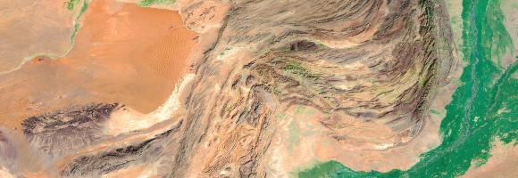
Humans need increasingly more biomass for food, fodder, fibre and energy. Meeting these demands changes global ecosystems. Tracking changes in total biomass production or land productivity is an essential part of monitoring land transformations that are typically associated with land degradation. Land productivity dynamics (LPD) are used as an indicator of change or stability of the land’s capacity to sustain primary production. This layer displays the areas of concern for land productivity related issues, derived from the convergence of global evidence of human-environment interactions that can have consequences on land degradation.

The GHS-BUILT-S spatial raster dataset depicts the distribution of the built-up (BU) surfaces estimates between 1975 and 2030 in 5 year intervals and two functional use components a) the total BU surface and b) the non-residential (NRES) BU surface. The data is made by spatial-temporal interpolation of five observed collections of multiple-sensor, multiple-platform satellite imageries: Landsat (MSS, TM, ETM sensor) data supports the 1975, 1990, 2000, and 2014 epochs, while a Sentinel-2 (S2) image composite (GHS-composite-S2 R2020A) supports the 2018 epoch.
This data represents the total BU surface (square meters) for year 1975 over cells of 1x1 km size.

The GHS-BUILT-S spatial raster dataset depicts the distribution of the built-up (BU) surfaces estimates between 1975 and 2030 in 5 year intervals and two functional use components a) the total BU surface and b) the non-residential (NRES) BU surface. The data is made by spatial-temporal interpolation of five observed collections of multiple-sensor, multiple-platform satellite imageries: Landsat (MSS, TM, ETM sensor) data supports the 1975, 1990, 2000, and 2014 epochs, while a Sentinel-2 (S2) image composite (GHS-composite-S2 R2020A) supports the 2018 epoch.
This data represents the total BU surface estimates (square meters) for year 1975 over cells of 100x100 m size.

The GHS-BUILT-S spatial raster dataset depicts the distribution of the built-up (BU) surfaces estimates between 1975 and 2030 in 5 year intervals and two functional use components a) the total BU surface and b) the non-residential (NRES) BU surface. The data is made by spatial-temporal interpolation of five observed collections of multiple-sensor, multiple-platform satellite imageries: Landsat (MSS, TM, ETM sensor) data supports the 1975, 1990, 2000, and 2014 epochs, while a Sentinel-2 (S2) image composite (GHS-composite-S2 R2020A) supports the 2018 epoch.
This data represents the total BU surface (square meters) for year 1980 over cells of 1x1 km size.

The GHS-BUILT-S spatial raster dataset depicts the distribution of the built-up (BU) surfaces estimates between 1975 and 2030 in 5 year intervals and two functional use components a) the total BU surface and b) the non-residential (NRES) BU surface. The data is made by spatial-temporal interpolation of five observed collections of multiple-sensor, multiple-platform satellite imageries: Landsat (MSS, TM, ETM sensor) data supports the 1975, 1990, 2000, and 2014 epochs, while a Sentinel-2 (S2) image composite (GHS-composite-S2 R2020A) supports the 2018 epoch.
This data represents the total BU surface estimates (square meters) for year 1980 over cells of 100x100 m size.

The GHS-BUILT-S spatial raster dataset depicts the distribution of the built-up (BU) surfaces estimates between 1975 and 2030 in 5 year intervals and two functional use components a) the total BU surface and b) the non-residential (NRES) BU surface. The data is made by spatial-temporal interpolation of five observed collections of multiple-sensor, multiple-platform satellite imageries: Landsat (MSS, TM, ETM sensor) data supports the 1975, 1990, 2000, and 2014 epochs, while a Sentinel-2 (S2) image composite (GHS-composite-S2 R2020A) supports the 2018 epoch.
This data represents the total BU surface (square meters) for year 1985 over cells of 1x1 km size.

The GHS-BUILT-S spatial raster dataset depicts the distribution of the built-up (BU) surfaces estimates between 1975 and 2030 in 5 year intervals and two functional use components a) the total BU surface and b) the non-residential (NRES) BU surface. The data is made by spatial-temporal interpolation of five observed collections of multiple-sensor, multiple-platform satellite imageries: Landsat (MSS, TM, ETM sensor) data supports the 1975, 1990, 2000, and 2014 epochs, while a Sentinel-2 (S2) image composite (GHS-composite-S2 R2020A) supports the 2018 epoch.
This data represents the total BU surface estimates (square meters) for year 1985 over cells of 100x100 m size.

The GHS-BUILT-S spatial raster dataset depicts the distribution of the built-up (BU) surfaces estimates between 1975 and 2030 in 5 year intervals and two functional use components a) the total BU surface and b) the non-residential (NRES) BU surface. The data is made by spatial-temporal interpolation of five observed collections of multiple-sensor, multiple-platform satellite imageries: Landsat (MSS, TM, ETM sensor) data supports the 1975, 1990, 2000, and 2014 epochs, while a Sentinel-2 (S2) image composite (GHS-composite-S2 R2020A) supports the 2018 epoch.
This data represents the total BU surface (square meters) for year 1990 over cells of 1x1 km size.

The GHS-BUILT-S spatial raster dataset depicts the distribution of the built-up (BU) surfaces estimates between 1975 and 2030 in 5 year intervals and two functional use components a) the total BU surface and b) the non-residential (NRES) BU surface. The data is made by spatial-temporal interpolation of five observed collections of multiple-sensor, multiple-platform satellite imageries: Landsat (MSS, TM, ETM sensor) data supports the 1975, 1990, 2000, and 2014 epochs, while a Sentinel-2 (S2) image composite (GHS-composite-S2 R2020A) supports the 2018 epoch.
This data represents the total BU surface estimates (square meters) for year 1990 over cells of 100x100 m size.

The GHS-BUILT-S spatial raster dataset depicts the distribution of the built-up (BU) surfaces estimates between 1975 and 2030 in 5 year intervals and two functional use components a) the total BU surface and b) the non-residential (NRES) BU surface. The data is made by spatial-temporal interpolation of five observed collections of multiple-sensor, multiple-platform satellite imageries: Landsat (MSS, TM, ETM sensor) data supports the 1975, 1990, 2000, and 2014 epochs, while a Sentinel-2 (S2) image composite (GHS-composite-S2 R2020A) supports the 2018 epoch.
This data represents the total BU surface (square meters) for year 1995 over cells of 1x1 km size.

The GHS-BUILT-S spatial raster dataset depicts the distribution of the built-up (BU) surfaces estimates between 1975 and 2030 in 5 year intervals and two functional use components a) the total BU surface and b) the non-residential (NRES) BU surface. The data is made by spatial-temporal interpolation of five observed collections of multiple-sensor, multiple-platform satellite imageries: Landsat (MSS, TM, ETM sensor) data supports the 1975, 1990, 2000, and 2014 epochs, while a Sentinel-2 (S2) image composite (GHS-composite-S2 R2020A) supports the 2018 epoch.
This data represents the total BU surface estimates (square meters) for year 1995 over cells of 100x100 m size.

The GHS-BUILT-S spatial raster dataset depicts the distribution of the built-up (BU) surfaces estimates between 1975 and 2030 in 5 year intervals and two functional use components a) the total BU surface and b) the non-residential (NRES) BU surface. The data is made by spatial-temporal interpolation of five observed collections of multiple-sensor, multiple-platform satellite imageries: Landsat (MSS, TM, ETM sensor) data supports the 1975, 1990, 2000, and 2014 epochs, while a Sentinel-2 (S2) image composite (GHS-composite-S2 R2020A) supports the 2018 epoch.
This data represents the total BU surface (square meters) for year 2000 over cells of 1x1 km size.

The GHS-BUILT-S spatial raster dataset depicts the distribution of the built-up (BU) surfaces estimates between 1975 and 2030 in 5 year intervals and two functional use components a) the total BU surface and b) the non-residential (NRES) BU surface. The data is made by spatial-temporal interpolation of five observed collections of multiple-sensor, multiple-platform satellite imageries: Landsat (MSS, TM, ETM sensor) data supports the 1975, 1990, 2000, and 2014 epochs, while a Sentinel-2 (S2) image composite (GHS-composite-S2 R2020A) supports the 2018 epoch.
This data represents the total BU surface estimates (square meters) for year 2000 over cells of 100x100 m size.

The GHS-BUILT-S spatial raster dataset depicts the distribution of the built-up (BU) surfaces estimates between 1975 and 2030 in 5 year intervals and two functional use components a) the total BU surface and b) the non-residential (NRES) BU surface. The data is made by spatial-temporal interpolation of five observed collections of multiple-sensor, multiple-platform satellite imageries: Landsat (MSS, TM, ETM sensor) data supports the 1975, 1990, 2000, and 2014 epochs, while a Sentinel-2 (S2) image composite (GHS-composite-S2 R2020A) supports the 2018 epoch.
This data represents the total BU surface (square meters) for year 2005 over cells of 1x1 km size.

The GHS-BUILT-S spatial raster dataset depicts the distribution of the built-up (BU) surfaces estimates between 1975 and 2030 in 5 year intervals and two functional use components a) the total BU surface and b) the non-residential (NRES) BU surface. The data is made by spatial-temporal interpolation of five observed collections of multiple-sensor, multiple-platform satellite imageries: Landsat (MSS, TM, ETM sensor) data supports the 1975, 1990, 2000, and 2014 epochs, while a Sentinel-2 (S2) image composite (GHS-composite-S2 R2020A) supports the 2018 epoch.
This data represents the total BU surface estimates (square meters) for year 2005 over cells of 100x100 m size.

The GHS-BUILT-S spatial raster dataset depicts the distribution of the built-up (BU) surfaces estimates between 1975 and 2030 in 5 year intervals and two functional use components a) the total BU surface and b) the non-residential (NRES) BU surface. The data is made by spatial-temporal interpolation of five observed collections of multiple-sensor, multiple-platform satellite imageries: Landsat (MSS, TM, ETM sensor) data supports the 1975, 1990, 2000, and 2014 epochs, while a Sentinel-2 (S2) image composite (GHS-composite-S2 R2020A) supports the 2018 epoch.
This data represents the total BU surface (square meters) for year 2010 over cells of 1x1 km size.

The GHS-BUILT-S spatial raster dataset depicts the distribution of the built-up (BU) surfaces estimates between 1975 and 2030 in 5 year intervals and two functional use components a) the total BU surface and b) the non-residential (NRES) BU surface. The data is made by spatial-temporal interpolation of five observed collections of multiple-sensor, multiple-platform satellite imageries: Landsat (MSS, TM, ETM sensor) data supports the 1975, 1990, 2000, and 2014 epochs, while a Sentinel-2 (S2) image composite (GHS-composite-S2 R2020A) supports the 2018 epoch.
This data represents the total BU surface estimates (square meters) for year 2010 over cells of 100x100 m size.

The GHS-BUILT-S spatial raster dataset depicts the distribution of the built-up (BU) surfaces estimates between 1975 and 2030 in 5 year intervals and two functional use components a) the total BU surface and b) the non-residential (NRES) BU surface. The data is made by spatial-temporal interpolation of five observed collections of multiple-sensor, multiple-platform satellite imageries: Landsat (MSS, TM, ETM sensor) data supports the 1975, 1990, 2000, and 2014 epochs, while a Sentinel-2 (S2) image composite (GHS-composite-S2 R2020A) supports the 2018 epoch.
This data represents the total BU surface (square meters) for year 2015 over cells of 1x1 km size.

The GHS-BUILT-S spatial raster dataset depicts the distribution of the built-up (BU) surfaces estimates between 1975 and 2030 in 5 year intervals and two functional use components a) the total BU surface and b) the non-residential (NRES) BU surface. The data is made by spatial-temporal interpolation of five observed collections of multiple-sensor, multiple-platform satellite imageries: Landsat (MSS, TM, ETM sensor) data supports the 1975, 1990, 2000, and 2014 epochs, while a Sentinel-2 (S2) image composite (GHS-composite-S2 R2020A) supports the 2018 epoch.
This data represents the total BU surface estimates (square meters) for year 2015 over cells of 100x100 m size.

The GHS-BUILT-S spatial raster dataset depicts the distribution of the built-up (BU) surfaces estimates between 1975 and 2030 in 5 year intervals and two functional use components a) the total BU surface and b) the non-residential (NRES) BU surface. The data is made by spatial-temporal interpolation of five observed collections of multiple-sensor, multiple-platform satellite imageries: Landsat (MSS, TM, ETM sensor) data supports the 1975, 1990, 2000, and 2014 epochs, while a Sentinel-2 (S2) image composite (GHS-composite-S2 R2020A) supports the 2018 epoch.
This data represents the total BU surface (square meters) for year 2020 over cells of 1x1 km size.

The GHS-BUILT-S spatial raster dataset depicts the distribution of the built-up (BU) surfaces estimates between 1975 and 2030 in 5 year intervals and two functional use components a) the total BU surface and b) the non-residential (NRES) BU surface. The data is made by spatial-temporal interpolation of five observed collections of multiple-sensor, multiple-platform satellite imageries: Landsat (MSS, TM, ETM sensor) data supports the 1975, 1990, 2000, and 2014 epochs, while a Sentinel-2 (S2) image composite (GHS-composite-S2 R2020A) supports the 2018 epoch.
This data represents the total BU surface estimates (square meters) for year 2020 over cells of 100x100 m size.

The GHS-BUILT-S spatial raster dataset depicts the distribution of the built-up (BU) surfaces estimates between 1975 and 2030 in 5 year intervals and two functional use components a) the total BU surface and b) the non-residential (NRES) BU surface. The data is made by spatial-temporal interpolation of five observed collections of multiple-sensor, multiple-platform satellite imageries: Landsat (MSS, TM, ETM sensor) data supports the 1975, 1990, 2000, and 2014 epochs, while a Sentinel-2 (S2) image composite (GHS-composite-S2 R2020A) supports the 2018 epoch.
This data represents the total BU surface estimates (square meters) for year 2025 over cells of 1x1 km size.

The GHS-BUILT-S spatial raster dataset depicts the distribution of the built-up (BU) surfaces estimates between 1975 and 2030 in 5 year intervals and two functional use components a) the total BU surface and b) the non-residential (NRES) BU surface. The data is made by spatial-temporal interpolation of five observed collections of multiple-sensor, multiple-platform satellite imageries: Landsat (MSS, TM, ETM sensor) data supports the 1975, 1990, 2000, and 2014 epochs, while a Sentinel-2 (S2) image composite (GHS-composite-S2 R2020A) supports the 2018 epoch.
This data represents the total BU surface estimates (square meters) for year 2025 over cells of 100x100 m size.

The GHS-BUILT-S spatial raster dataset depicts the distribution of the built-up (BU) surfaces estimates between 1975 and 2030 in 5 year intervals and two functional use components a) the total BU surface and b) the non-residential (NRES) BU surface. The data is made by spatial-temporal interpolation of five observed collections of multiple-sensor, multiple-platform satellite imageries: Landsat (MSS, TM, ETM sensor) data supports the 1975, 1990, 2000, and 2014 epochs, while a Sentinel-2 (S2) image composite (GHS-composite-S2 R2020A) supports the 2018 epoch.
This data represents the total BU surface estimates (square meters) for year 2030 over cells of 1x1 km size.

The GHS-BUILT-S spatial raster dataset depicts the distribution of the built-up (BU) surfaces estimates between 1975 and 2030 in 5 year intervals and two functional use components a) the total BU surface and b) the non-residential (NRES) BU surface. The data is made by spatial-temporal interpolation of five observed collections of multiple-sensor, multiple-platform satellite imageries: Landsat (MSS, TM, ETM sensor) data supports the 1975, 1990, 2000, and 2014 epochs, while a Sentinel-2 (S2) image composite (GHS-composite-S2 R2020A) supports the 2018 epoch.
This data represents the total BU surface estimates (square meters) for year 2030 over cells of 1x1 km size.

The GHS-BUILT-S spatial raster dataset depicts the distribution of the built-up (BU) surfaces estimates between 1975 and 2030 in 5 year intervals and two functional use components a) the total BU surface and b) the non-residential (NRES) BU surface. The data is made by spatial-temporal interpolation of five observed collections of multiple-sensor, multiple-platform satellite imageries: Landsat (MSS, TM, ETM sensor) data supports the 1975, 1990, 2000, and 2014 epochs, while a Sentinel-2 (S2) image composite (GHS-composite-S2 R2020A) supports the 2018 epoch.
This data represents the total BU surface estimates (square meters) for year 2030 over cells of 100x100 m size.

The GHS-BUILT-S spatial raster dataset depicts the distribution of the built-up (BU) surfaces estimates between 1975 and 2030 in 5 year intervals and two functional use components a) the total BU surface and b) the non-residential (NRES) BU surface. The data is made by spatial-temporal interpolation of five observed collections of multiple-sensor, multiple-platform satellite imageries: Landsat (MSS, TM, ETM sensor) data supports the 1975, 1990, 2000, and 2014 epochs, while a Sentinel-2 (S2) image composite (GHS-composite-S2 R2020A) supports the 2018 epoch.
This data represents the total BU surface estimates (square meters) for year 2030 over cells of 100x100 m size.

The GHS-BUILT-S spatial raster dataset depicts the distribution of the built-up (BU) surfaces estimates between 1975 and 2030 in 5 year intervals and two functional use components a) the total BU surface and b) the non-residential (NRES) BU surface. The data is made by spatial-temporal interpolation of five observed collections of multiple-sensor, multiple-platform satellite imageries: Landsat (MSS, TM, ETM sensor) data supports the 1975, 1990, 2000, and 2014 epochs, while a Sentinel-2 (S2) image composite (GHS-composite-S2 R2020A) supports the 2018 epoch.
This data represents the Non Residential BU surface estimates (square meters) for year 2030 over cells of 100 x100 m size.

The GHS-BUILT-S spatial raster dataset depicts the distribution of the built-up (BU) surfaces estimates between 1975 and 2030 in 5 year intervals and two functional use components a) the total BU surface and b) the non-residential (NRES) BU surface. The data is made by spatial-temporal interpolation of five observed collections of multiple-sensor, multiple-platform satellite imageries: Landsat (MSS, TM, ETM sensor) data supports the 1975, 1990, 2000, and 2014 epochs, while a Sentinel-2 (S2) image composite (GHS-composite-S2 R2020A) supports the 2018 epoch.
This data represents the Non residential BU surface estimates (square meters) for year 2030 over cells of 1x1 km size.
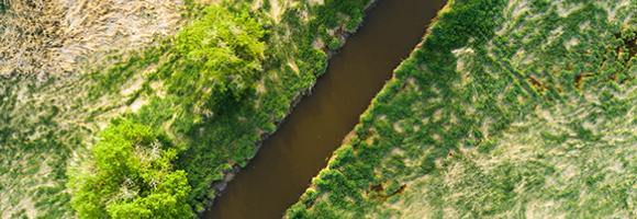

In 2020, a group of researchers carried out analysis to examine the importance of Indigenous Peoples’ lands for preserving Intact Forest Landscapes.(Fa et al.2020)They used geospatial data on the extent of Indigenous Peoples’ lands reported by Garnett et al. (2018), and Geospatial data for IFLs were sourced from the Intact Forest Landscapes website (www.intactforests.org) for the years 2000, 2013, and 2016 (Potapov et al. 2017)In the paper they have shown that the proportion of Indigenous Peoples’ lands mapped as IFLs was considerably higher (10.9%) than the proportion of other lands (defined here as all land outside Indigenous Peoples’ lands) mapped as IFLs (6.8%).
In this map we reported the percentage of Intact Forest Lansdcapes reduction in Indigenous People Lands for the period 2000-2016. IN the table we reported also the percentage of IFLs reduction in other lands. To explore more IFLs conservation strategies for African, Caribbean and Pacific countries you can check BIOPAMA Geonode Layers
Sources:
Fa JE, Watson JE, Leiper I, Potapov P, Evans TD, Burgess ND, Molnár Z, Fernández‐Llamazares Á, Duncan T, Wang S, Austin BJ. Importance of Indigenous Peoples’ lands for the conservation of Intact Forest Landscapes. Frontiers in Ecology and the Environment. 2020 Apr;18(3):135-4
Land cover is defined as the physical material at the surface of the earth, usually documented via the interpretation of earth observations. Common land cover types include trees, grass, bare ground, built up areas, water, etc. How well are different ecosystem types (as indicated by land cover) preserved and how strong are anthropogenic changes affecting their distribution in a given area? Human pressures are constantly increasing and it is important to monitor the consequences of the associated changes on the environment. This map shows the changes in land cover between 1995 and 2015.

Humans need increasingly more biomass for food, fodder, fiber and energy. In Africa, circa 22% of the vegetated land surface showed a decline or unstable land productivity between 1999 and 2013. Persistent reduction of land productivity points to long-term alteration of the health and productive capacity of the land, which are characteristic of land degradation. It has impact on ecosystem services and benefits, thus on the sustainable livelihoods of human communities. This map shows the dynamics of (vegetated) land productivity over a time period, in other terms the trajectories of above-ground biomass. It reflects changes in ecosystem functioning e.g. vegetation growth cycles due to natural variation and/or human intervention, and can be associated with processes of land degradation or recovery. The 5 classes depict two levels of persistent productivity decline, one level of instability or stress in capacity, one level of stable productivity and one level of increased productivity.
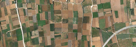
Habitat fragmentation occurs when natural habitat is broken up by non-natural land uses. For this layer, land fragmentation is expressed as the Natural Land Cover Pattern Index (NLPI), which classifies natural or semi-natural landcover into six spatial pattern classes: core, edge, perforation, islet, margin, and core-opening. Natural landcover pixels from Climate Change Initiative Land Cover (CCI-LC) raster maps are classified as ‘core’ habitat. Non-natural land cover pixels within core habitat are classified as ‘core openings’ as these represent openings from within natural habitat. External interfaces between core and non-natural landcover are classified as ‘edges’ (i.e. exposed to outside-in habitat loss pressures), while internal interfaces between core and core-openings are classified as ‘perforations’ (i.e. exposed to inside-out habitat loss pressure). Collections of isolated natural landcover pixels that are too small to contain core habitat are classified as ‘islets’, while similarly small collections of pixels are classified as ‘margins’ when they are connected to core habitats.
Humans need increasingly more biomass for food, fodder, fiber and energy. In Africa, circa 22% of the vegetated land surface showed a decline or unstable land productivity between 1999 and 2013. Persistent reduction of land productivity points to long-term alteration of the health and productive capacity of the land, which are characteristic of land degradation. It has impact on ecosystem services and benefits, thus on the sustainable livelihoods of human communities. This map shows the dynamics of (vegetated) land productivity over a time period, in other terms the trajectories of above-ground biomass. It reflects changes in ecosystem functioning e.g. vegetation growth cycles due to natural variation and/or human intervention, and can be associated with processes of land degradation or recovery. The 5 classes depict two levels of persistent productivity decline, one level of instability or stress in capacity, one level of stable productivity and one level of increased productivity.

Monitoring of sea surface temperature (SST) provides fundamental information on the global climate system and for the study of marine ecosystems. This layer compares the SST value of the last full month with the long-term mean SST. A positive anomaly (warm colours) means the monthly SST is warmer than the long-term average for that month; a negative anomaly (cool colours) means it is cooler than the average.

Monitoring of sea surface temperature (SST) provides fundamental information on the global climate system and for the study of marine ecosystems. For example, it helps estimating heat stress conducive to coral bleaching, the process by which they expel the symbiotic algae living in their tissues and become white (bleached) and vulnerable. The NOAA Coral Reef Watch's daily global 5km satellite SST Anomaly (SSTA) compares the daily SST value with the long-term mean SST. A positive anomaly (+1.0 °C or more, warm colours) means the daily SST is warmer than the long-term average for that day; a negative anomaly (-1.0 °C or less, cold colours) means it is cooler than the average.
Ocean temperature is related to ocean heat content (the energy absorbed by the ocean), an important topic in the study of global warming. Monitoring of sea surface temperature (SST) from earth-orbiting infrared radiometers has had a wide impact on oceanographic science. It provides fundamental information on the global climate system and for the study of marine ecosystems. For example, it helps estimating heat stress conducive to coral bleaching, the process by which they expel the symbiotic algae living in their tissues and become white (bleached) and vulnerable. The NOAA Coral Reef Watch Daily Global 5km Satellite Sea Surface Temperature product (a.k.a. CoralTemp) measures the night-time ocean temperature at the sea surface, calibrated to 0.2 meters depth.
Monitoring of sea surface temperature (SST) provides fundamental information on the global climate system and for the study of marine ecosystems. For example, it helps estimating heat stress conducive to coral bleaching, the process by which they expel the symbiotic algae living in their tissues and become white (bleached) and vulnerable. The NOAA Coral Reef Watch's daily global 5km 7-day SST Trend product shows the SST trend for the most recent seven days. Pixels coloured in blue to purple follow a cooling trend while pixels coloured in yellow to red follow a warming trend. Pixels coloured in green have insignificant trends.
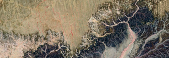
Organisms and non-living elements of the environment such as climate, soil, and water are connected through the movement of nutrients and energy in ecosystems. Ecosystems represent specific areas where organisms and environmental conditions create a network of interactions and are affected by forces such as disturbance (temporary change in environmental conditions that causes a pronounced change) and succession (process of change in the species structure of an ecological community over time). This layer maps the Ecosystems of Africa, based on Africa's climate regions, topography and lithology (bedrock), with a 100m spatial resolution.
This dataset provides a continent-wide, raster-based spatial representation of Earth's surface heat flow across the African tectonic plate for the year 2013, modeled under a historical baseline scenario. The data quantifies the amount of thermal energy moving from the Earth's interior to its surface, with values explicitly expressed in watts per square meter (W/m²). This resource is critical for identifying geothermal potential, understanding tectonic anomalies, and supporting broader geoscientific and energy research.
Sources and ContextThis layer is part of the Geothermal Atlas for Africa developed within the LEAP-RE project
This dataset comprises a collection of shapefiles detailing the geographical locations and attributes of various wells across Africa, with a strong focus on geothermal exploration and assessment. Together, these layers offer a valuable resource for geothermal energy planning, subsurface geological analysis, and infrastructure mapping. The collection includes the following spatial data layers:
These layers are part of the Geothermal Atlas for Africa developed within the LEAP-RE project"
This dataset compiles geophysical models detailing the thickness of the Earth's outer layers, ranging from surface sedimentary basins down to the base of the lithosphere. The collection serves a dual purpose: it provides broad, global baseline data for sediment distribution, while also offering high-resolution, integrated regional models specifically focused on the African plate.
Dataset Contents:
I. Global Baselines
II. African Regional Models
These layers are part of the Geothermal Atlas for Africa developed within the LEAP-RE project
This dataset shows the location of hydrocarbon provinces with proven petroleum reserves. This data was compiled as part of the USGS's World Energy Project (WEP).
This dataset is part of the LEAP-RE project collection. For more information visit https://www.leap-re.eu/

Higher energy demands in Africa has led to a wide expansion of the number of hydropower sites, mainly between the 1960s and 1980s. The construction of dams causes impoundments of rivers and reservoirs in the regions of dam influence, with higher evaporation and water temperatures due to increased water surfaces. This map shows the he surface area (sqkm) of African reservoirs subject to hydropower production for the year 2016. It includes reservoirs of associated hydropower plants with installed capacities above 5MW. Apart from this, only reservoirs with a detected dam-caused impoundment of water surface are considered.
Development test dataset: random 0-100 values on the 0.35° Nature Africa grid clipped to the DRC. Not real data.