Conservation Tracking

RCoE Action

Topic

Policy

Target

Title

Map showing the average continental surface temperature of the year 2022. This map was created by interpolating raw monthly satellite data to fill holes in the grids and subsequently adding and averaging the monthly surface temperatures of the year 2022. The data is clipped to only show the African continental region. The raw data is collected during the daytime by the Moderate Resolution Imaging Spectroradiometer (MODIS), an instrument on NASA's Terra and Aqua satellites. Please note that the type of "surface" MODIS measures varies as a function of location. In some places, the measurement represents the skin temperature of the bare land surface. In other places, the temperature represents the skin temperature of whatever is on the land-including snow and ice, or the leafy canopy of forests and crop fields, or human-made structures such as pavement and building rooftops.
Values are expressed in °C.
This dataset is part of the LEAP-RE project collection. For more information visit https://www.leap-re.eu/

The tool highlights locations where the local association between piped water access and the selected nutrition indicator is both negative and statistically significant. In this application, priority areas are further restricted to locations where piped water access is below 80%, ensuring that the results remain relevant for policy intervention.

The identified areas are classified as having strong, moderate, or mild associations according to the magnitude of the local GWR coefficient. This classification helps users determine the appropriate intensity of intervention. The spatially varying coefficients therefore allow users to identify areas where limited piped water access is most strongly associated with poorer nutritional outcomes among children under five, supporting targeted interventions, programme planning, and place-based development strategies.

Monitoring of sea surface temperature (SST) provides fundamental information on the global climate system and for the study of marine ecosystems. For example, it helps estimating heat stress conducive to coral bleaching, the process by which they expel the symbiotic algae living in their tissues and become white (bleached) and vulnerable. The NOAA Coral Reef Watch's daily global 5km satellite SST Anomaly (SSTA) compares the daily SST value with the long-term mean SST. A positive anomaly (+1.0 °C or more, warm colours) means the daily SST is warmer than the long-term average for that day; a negative anomaly (-1.0 °C or less, cold colours) means it is cooler than the average.

Ocean temperature is related to ocean heat content (the energy absorbed by the ocean), an important topic in the study of global warming. Monitoring of sea surface temperature (SST) from earth-orbiting infrared radiometers has had a wide impact on oceanographic science. It provides fundamental information on the global climate system and for the study of marine ecosystems. For example, it helps estimating heat stress conducive to coral bleaching, the process by which they expel the symbiotic algae living in their tissues and become white (bleached) and vulnerable. The NOAA Coral Reef Watch Daily Global 5km Satellite Sea Surface Temperature product (a.k.a. CoralTemp) measures the night-time ocean temperature at the sea surface, calibrated to 0.2 meters depth.

Monitoring of sea surface temperature (SST) provides fundamental information on the global climate system and for the study of marine ecosystems. For example, it helps estimating heat stress conducive to coral bleaching, the process by which they expel the symbiotic algae living in their tissues and become white (bleached) and vulnerable. The NOAA Coral Reef Watch's daily global 5km 7-day SST Trend product shows the SST trend for the most recent seven days. Pixels coloured in blue to purple follow a cooling trend while pixels coloured in yellow to red follow a warming trend. Pixels coloured in green have insignificant trends.

"This map shows, for each grid cell, the environmental impact in terms of CO₂-equivalent emissions per kilowatt-hour [g CO2 eq/kWh] generated by by the following systems:

Cooling Absorption System;
Refrigeration Absorption System;
Binary ORC Power Plant;
Flash Power Plant;
Heat for Direct Use;
Heat for High Temperature Heat Pump;

The maps refer to:

base case scenario;
upside scenario, modelling a better fluid flow;
up up side, modelling both better fluid flow and higher underground temperatures.

This layer is part of the Geothermal Atlas for Africa developed within the LEAP-RE project"

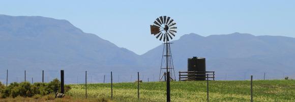
Increasing water scarcity and water quality issues are serious constraints, especially for Northern Africa. A comprehensive assessment of spatial and temporal precipitation frequency is the initial step for defining public policies relating to water resources management and environmental monitoring. In the agricultural sector, a detailed knowledge of precipitation patterns is necessary to identify the most appropriate crop varieties for the region and to effectively manage climate related uncertainties. Precipitation frequency is also a central source of information for hazard mitigation and management. This layer shows the average annual precipitation (mm/year) for the period 1981-2017 across the continent.

This dataset provides fixed broadband performance metrics in zoom level 16 web Mercator tiles (approximately 610.8 meters by 610.8 meters at the equator). Download speed is collected via the Speedtest by Ookla applications for Android and iOS and averaged for each tile. Measurements are filtered to results containing GPS-quality location accuracy. Speedtest data is used today by commercial fixed network operators around the world to inform network buildout, improve global Internet quality, and increase Internet accessibility. This data can be used for rural and urban connectivity development, to help make the internet better, faster, and more accessible for everyone.

The GHS-BUILT-S spatial raster dataset depicts the distribution of the built-up (BU) surfaces estimates between 1975 and 2030 in 5 year intervals and two functional use components a) the total BU surface and b) the non-residential (NRES) BU surface. The data is made by spatial-temporal interpolation of five observed collections of multiple-sensor, multiple-platform satellite imageries: Landsat (MSS, TM, ETM sensor) data supports the 1975, 1990, 2000, and 2014 epochs, while a Sentinel-2 (S2) image composite (GHS-composite-S2 R2020A) supports the 2018 epoch.

This data represents the total BU surface (square meters) for year 1975 over cells of 1x1 km size.

This data represents the total BU surface estimates (square meters) for year 1975 over cells of 100x100 m size.

This data represents the total BU surface (square meters) for year 1980 over cells of 1x1 km size.

This data represents the total BU surface estimates (square meters) for year 1980 over cells of 100x100 m size.

This data represents the total BU surface (square meters) for year 1985 over cells of 1x1 km size.

This data represents the total BU surface estimates (square meters) for year 1985 over cells of 100x100 m size.

This data represents the total BU surface (square meters) for year 1990 over cells of 1x1 km size.

This data represents the total BU surface estimates (square meters) for year 1990 over cells of 100x100 m size.

This data represents the total BU surface (square meters) for year 1995 over cells of 1x1 km size.

This data represents the total BU surface estimates (square meters) for year 1995 over cells of 100x100 m size.

This data represents the total BU surface (square meters) for year 2000 over cells of 1x1 km size.

This data represents the total BU surface estimates (square meters) for year 2000 over cells of 100x100 m size.

This data represents the total BU surface (square meters) for year 2005 over cells of 1x1 km size.

This data represents the total BU surface estimates (square meters) for year 2005 over cells of 100x100 m size.

This data represents the total BU surface (square meters) for year 2010 over cells of 1x1 km size.

This data represents the total BU surface estimates (square meters) for year 2010 over cells of 100x100 m size.

This data represents the total BU surface (square meters) for year 2015 over cells of 1x1 km size.

This data represents the total BU surface estimates (square meters) for year 2015 over cells of 100x100 m size.

This data represents the total BU surface (square meters) for year 2020 over cells of 1x1 km size.

This data represents the total BU surface estimates (square meters) for year 2020 over cells of 100x100 m size.

This data represents the total BU surface estimates (square meters) for year 2025 over cells of 1x1 km size.

This data represents the total BU surface estimates (square meters) for year 2025 over cells of 100x100 m size.

This data represents the total BU surface estimates (square meters) for year 2030 over cells of 1x1 km size.

This data represents the total BU surface estimates (square meters) for year 2030 over cells of 100x100 m size.

This data represents the Non Residential BU surface estimates (square meters) for year 2030 over cells of 100 x100 m size.

This data represents the Non residential BU surface estimates (square meters) for year 2030 over cells of 1x1 km size.

The hydropower installed capacity indicates the amount of energy a hydropower plant can produce in its turbines. In 2016, hydropower accounted for 54% of the installed capacity in Eastern Africa, 58% in Central Africa and 30% in Western Africa with fourteen countries having a hydropower share above 50% and eight countries above 70%. These highly hydropower-dependent countries are particularly prone to electricity cuts due to the lack of water caused by severe droughts. This map shows the location and installed capacities of hydropower plants above 5MW installed capacity in Africa for year 2016, representing 95% of the total hydropower installed capacity in Africa.

Higher energy demands in Africa has led to a wide expansion of the number of hydropower sites, mainly between the 1960s and 1980s. The construction of dams causes impoundments of rivers and reservoirs in the regions of dam influence, with higher evaporation and water temperatures due to increased water surfaces. This map shows the he surface area (sqkm) of African reservoirs subject to hydropower production for the year 2016. It includes reservoirs of associated hydropower plants with installed capacities above 5MW. Apart from this, only reservoirs with a detected dam-caused impoundment of water surface are considered.

This layer provides estimates of the percentage of children aged 2 to 10 years (PfPR2–10) with detectable Plasmodium falciparum parasites in 2022. The estimates are generated using geostatistical models based on point prevalence surveys, routine surveillance data, and a wide range of geospatial covariates representing mosquito habitat and environmental conditions. The data are available annually from 2000 onward, covering all malaria-endemic countries, at a spatial resolution of 5 × 5 km.

This dataset provides mobile (cellular) network performance metrics in zoom level 16 web Mercator tiles (approximately 610.8 meters by 610.8 meters at the equator). Download speed is collected via the Speedtest by Ookla applications for Android and iOS and averaged for each tile. Measurements are filtered to results containing GPS-quality location accuracy. Speedtest data is used today by commercial mobile network operators around the world to inform network buildout, improve global Internet quality, and increase Internet accessibility. This data can be used for rural and urban connectivity development, to help make the internet better, faster, and more accessible for everyone.

This dataset compiles global and regional models of the Mohorovičić discontinuity (Moho) depth from 2019 to 2022, providing key insights into crustal thickness and lithospheric boundaries. All layer values are expressed in kilometers (km). It includes the Moho Depth (Finger et al., 2022) map, which details the boundary derived from S-wave seismic tomography data, alongside its corresponding Moho Depth Uncertainty layer to highlight spatial confidence and data reliability. Additionally, it features the Global Moho Depth (Szwillus et al., 2019) map, derived using a nonstationary kriging algorithm (Risser & Calder, 2017), which serves as an excellent comparative baseline for structural, geophysical, and tectonic analysis.

These layers are part of the Geothermal Atlas for Africa developed within the LEAP-RE project

Priority areas are identified using local coefficients estimated through Geographically Weighted Regression (GWR), which measures the spatially varying relationship between access to Water infrastructure and education using the indicator of percentage of population with secondary education. The tool highlights locations where the local association between access to piped water s and the selected education indicator is both negative and statistically significant. The identified areas are classified as having strong, moderate, or mild associations according to the magnitude of the local GWR coefficient. This classification helps users determine the appropriate intensity of intervention. The spatially varying coefficients therefore allow users to identify areas where limited sanitation access is most strongly associated with lower education, supporting targeted interventions, programme planning, and place-based development strategies.

Priority areas are identified using local coefficients estimated through Geographically Weighted Regression (GWR), which measures the spatially varying relationship between access to water infrastructure and gender using the indicator of percentage of women with secondary education. The tool highlights locations where the local association between access to piped water and the selected gender indicator is both negative and statistically significant. The identified areas are classified as having strong, moderate, or mild associations according to the magnitude of the local GWR coefficient. This classification helps users determine the appropriate intensity of intervention. The spatially varying coefficients therefore allow users to identify areas where limited water access is most strongly associated with lower women education, supporting targeted interventions, programme planning, and place-based development strategies.

Priority areas are identified using local coefficients estimated through Geographically Weighted Regression (GWR), which measures the spatially varying relationship between access to water infrastructure and health using the indicator of under 5 mortality. The tool highlights locations where the local association between access to piped water and the selected health indicator is both negative and statistically significant. The identified areas are classified as having strong, moderate, or mild associations according to the magnitude of the local GWR coefficient. This classification helps users determine the appropriate intensity of intervention. The spatially varying coefficients therefore allow users to identify areas where limited access to piped water is most strongly associated with higher child mortality, supporting targeted interventions, programme planning, and place-based development strategies.

Surface water affects many aspects of our world: the exchange of heat, gas and water vapour between the planet's surface and atmosphere. Water is the engine behind the distribution, movement and migration of Earth's plant and animal life and is just as essential for humans. It affects our capacity to grow crops and manage animal grazing lands, to run our industrial processes, to manufacture goods, it influences the movement of disease-vectors, toxins and pollutants, it generates energy directly (hydroelectric) and indirectly (thermoelectric), it is an essential part of our transport network, and forms part of our recreational, cultural and sporting world. The Water Occurrence dataset shows where surface water occurred between 1984 and 2018. Open water is any stretch of water open to the sky, and includes both freshwater and saltwater. The map displays water surfaces greater than 30m2 that are visible from space, including natural (rivers, lakes, coastal margins and wetlands) and artificial water bodies (reservoirs formed by dams, flooded areas such as opencast mines and quarries, flood irrigation areas such as paddy fields, and water bodies created by hydro-engineering projects such as waterway and harbour construction). This product captures both the intra and inter-annual variability and changes. The permanent water surfaces (100% occurrence over 36 years) are represented in blue, and areas where water sometimes occurs are shown in shades of pink to purple (0% < occurrence < 100%). The paler shades are areas where the water occurs less frequently. The map can support better informed water-management decision-making.

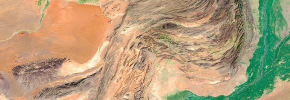
Water is a critical natural resource for both natural ecosystems and human subsistence. Some of the most immediate pressures on land that lead to degradation include diversion of surface waters and the removal of groundwater reserves to meet agricultural, industrial and domestic demands. This layer displays the areas of concern for water use related issues derived from the convergence of global evidence of human-environment interactions that can have consequences on land degradation. It highlights areas where the total water withdrawal (by the agriculture, industrial and domestic sectors) exceeds 40% of the total available annual renewable water supply.

The African Development Corridors Database (ADCD) is a comprehensive, georeferenced database detailing 79 ongoing and planned investment corridors across Africa, synthesizing data on 184 specific infrastructure projects (railways, ports, pipelines, airports, techno-cities, and industrial parks). Its purpose is to allow for critical assessment of the spatial and temporal impacts of massive infrastructure investments to maximize development opportunities and support the UN Sustainable Development Goals and AU Agenda 2063. The database includes 22 interlinked tabular and spatial attributes with provided sources, which is expected to improve coordination, efficiency, strategic planning, transparency, and impact assessments for governments, investment banks, practitioners, and conservationists, among other stakeholders.

This dataset provides the P50 projections for a geothermal system utilizing a Chiller unit.

Chiller refers to an absorption chiller or heat pump integrated into the geothermal system. It is used to provide cooling (by utilizing the geothermal heat) or to extract additional heat from the return fluid, thereby increasing the system's overall thermal harvest.

P50 is a statistical term used in risk analysis and forecasting. P50 represents the median scenario, meaning there is a 50% probability that the actual outcome will be higher than this value and a 50% probability it will be lower. It serves as the baseline "best estimate."

Metrics Definitions

Coefficient of Performance (COP) [-]: A measure of efficiency, defined as the ratio of useful heating or cooling provided to the work (energy) required to operate the Chiller. Higher values indicate greater efficiency.
Doublet Net Production [MW]: The actual useful power output (Megawatts) generated by the "doublet" (one production well + one injection well), subtracting any energy used by pumps or auxiliary equipment.
Levelized Cost of Energy (LCOE) [US$ct/kWh]: The average revenue per unit of energy needed to recover the cost of building and operating the plant over its entire life cycle. It essentially represents the break-even price.
Net Present Value (NPV) [million US$]: The current financial value of all future cash flows the project will generate, minus the initial investment costs. A positive NPV generally indicates a profitable project.
Optimized Depth of the Aquifer [m]: The calculated ideal drilling depth (meters) to reach the geothermal reservoir that balances drilling costs with temperature/flow benefits.
Pressure needed to drive pumps [Bar]: The total pressure difference required to drive the thermal loop through the reservoir and wellbore.
Production Flow Rate [m³/h]: The volume of geothermal fluid extracted from the reservoir per hour (cubic meters per hour).
Temperature at Reservoir [°C]: The natural temperature (Celsius) of the geothermal fluid within the subsurface rock formation before it is brought to the surface.
Transmissivity [Dm]: A measure of how easily fluid flows through the porous aquifer. It is the product of hydraulic conductivity and aquifer thickness (often measured in Darcy-meters). High transmissivity means easier extraction.
Well Distance [m]: The physical distance (meters) between the production well (extraction) and the injection well (return). Proper spacing prevents "short-circuiting," where cool injected water lowers the temperature of the production well too quickly.

These layers are part of the Geothermal Atlas for Africa developed within the LEAP-RE project

This dataset provides the P50 projections for a Direct Heat geothermal system.

Direct Heat refers to the use of geothermal energy for applications such as space heating, industrial processes, or agriculture. In the utilized model, it is assumed a minimum production temperature of at least 60°C and a reinjection temperature of 40°C.

Metrics Definitions

Coefficient of Performance (COP) [-]: A measure of efficiency, defined as the ratio of useful heating or cooling provided to the work (energy) required to operate the Chiller. Higher values indicate greater efficiency.
Doublet Net Production [MW]: The actual useful power output (Megawatts) generated by the ""doublet"" (one production well + one injection well), subtracting any energy used by pumps or auxiliary equipment.
Levelized Cost of Energy (LCOE) [US$ct/kWh]: The average revenue per unit of energy needed to recover the cost of building and operating the plant over its entire life cycle. It essentially represents the break-even price.
Net Present Value (NPV) [million US$]: The current financial value of all future cash flows the project will generate, minus the initial investment costs. A positive NPV generally indicates a profitable project.
Optimized Depth of the Aquifer [m]: The calculated ideal drilling depth (meters) to reach the geothermal reservoir that balances drilling costs with temperature/flow benefits.
Pressure needed to drive pumps [Bar]: The total pressure difference required to drive the thermal loop through the reservoir and wellbore.
Production Flow Rate [m³/h]: The volume of geothermal fluid extracted from the reservoir per hour (cubic meters per hour).
Temperature at Reservoir [°C]: The natural temperature (Celsius) of the geothermal fluid within the subsurface rock formation before it is brought to the surface.
Transmissivity [Dm]: A measure of how easily fluid flows through the porous aquifer. It is the product of hydraulic conductivity and aquifer thickness (often measured in Darcy-meters). High transmissivity means easier extraction.
Well Distance [m]: The physical distance (meters) between the production well (extraction) and the injection well (return). Proper spacing prevents ""short-circuiting,"" where cool injected water lowers the temperature of the production well too quickly.

This layer is part of the Geothermal Atlas for Africa developed within the LEAP-RE project

This dataset provides the P50 projections for a Direct Heat with Heat Pump geothermal system.

Direct Heat with Heat Pump refers to a scenario where a geothermal system is integrated with an industrial heat pump to upgrade low-grade heat. This allows for production from geothermal temperatures as low as 40°C, which are then heated by the pump to a delivery temperature of 80°C. The reinjection temperature is set to the production temperature minus 20°C, with a absolute minimum of 15°C.

Metrics Definitions

Coefficient of Performance (COP) [-]: A measure of efficiency, defined as the ratio of useful heating or cooling provided to the work (energy) required to operate the Chiller. Higher values indicate greater efficiency.
Doublet Net Production [MW]: The actual useful power output (Megawatts) generated by the ""doublet"" (one production well + one injection well), subtracting any energy used by pumps or auxiliary equipment.
Levelized Cost of Energy (LCOE) [US$ct/kWh]: The average revenue per unit of energy needed to recover the cost of building and operating the plant over its entire life cycle. It essentially represents the break-even price.
Net Present Value (NPV) [million US$]: The current financial value of all future cash flows the project will generate, minus the initial investment costs. A positive NPV generally indicates a profitable project.
Optimized Depth of the Aquifer [m]: The calculated ideal drilling depth (meters) to reach the geothermal reservoir that balances drilling costs with temperature/flow benefits.
Pressure needed to drive pumps [Bar]: The total pressure difference required to drive the thermal loop through the reservoir and wellbore.
Production Flow Rate [m³/h]: The volume of geothermal fluid extracted from the reservoir per hour (cubic meters per hour).
Temperature at Reservoir [°C]: The natural temperature (Celsius) of the geothermal fluid within the subsurface rock formation before it is brought to the surface.
Transmissivity [Dm]: A measure of how easily fluid flows through the porous aquifer. It is the product of hydraulic conductivity and aquifer thickness (often measured in Darcy-meters). High transmissivity means easier extraction.
Well Distance [m]: The physical distance (meters) between the production well (extraction) and the injection well (return). Proper spacing prevents ""short-circuiting,"" where cool injected water lowers the temperature of the production well too quickly.

This layer is part of the Geothermal Atlas for Africa developed within the LEAP-RE project

This dataset provides the P50 projections for an Organic Rankine Cycle (ORC) geothermal power plant.

Organic Rankine Cycle (ORC) refers to a binary power plant configuration where geothermal fluid (brine) is used to heat a secondary organic working fluid. This process allows for efficient electricity generation from medium-to-low temperature resources (typically 90°C to 150°C). The organic fluid vaporizes, drives a turbine, and is then condensed back into a liquid to repeat the cycle. The geothermal brine is reinjected into the reservoir after passing through the heat exchanger.

Metrics Definitions

Coefficient of Performance (COP) [-]: A measure of efficiency, defined as the ratio of useful heating or cooling provided to the work (energy) required to operate the Chiller. Higher values indicate greater efficiency.
Doublet Net Production [MW]: The actual useful power output (Megawatts) generated by the ""doublet"" (one production well + one injection well), subtracting any energy used by pumps or auxiliary equipment.
Levelized Cost of Energy (LCOE) [US$ct/kWh]: The average revenue per unit of energy needed to recover the cost of building and operating the plant over its entire life cycle. It essentially represents the break-even price.
Net Present Value (NPV) [million US$]: The current financial value of all future cash flows the project will generate, minus the initial investment costs. A positive NPV generally indicates a profitable project.
Optimized Depth of the Aquifer [m]: The calculated ideal drilling depth (meters) to reach the geothermal reservoir that balances drilling costs with temperature/flow benefits.
Pressure needed to drive pumps [Bar]: The total pressure difference required to drive the thermal loop through the reservoir and wellbore.
Production Flow Rate [m³/h]: The volume of geothermal fluid extracted from the reservoir per hour (cubic meters per hour).
Temperature at Reservoir [°C]: The natural temperature (Celsius) of the geothermal fluid within the subsurface rock formation before it is brought to the surface.
Transmissivity [Dm]: A measure of how easily fluid flows through the porous aquifer. It is the product of hydraulic conductivity and aquifer thickness (often measured in Darcy-meters). High transmissivity means easier extraction.
Well Distance [m]: The physical distance (meters) between the production well (extraction) and the injection well (return). Proper spacing prevents ""short-circuiting,"" where cool injected water lowers the temperature of the production well too quickly.

This layer is part of the Geothermal Atlas for Africa developed within the LEAP-RE project

Based on the Geothermal Atlas for Africa , the temperature models at 1 km, 2 km, 3 km, and 4 km depth are part of a 3D conductive thermal model of the African lithosphere.

These layers can be described as follows:

Model Basis: The layers are derived from a 3D grid with a vertical resolution of 250 meters down to 15 km, constructed using a lithosphere-scale conductive mode. This model incorporates sediment thickness, heat flow, crustal structure, and the depth of the Lithosphere-Asthenosphere Boundary (LAB).
Calibration: The models are calibrated using a dataset of 923 filtered temperature observations from the British Geological Survey, which were averaged per model grid cell to improve data assimilation.
Environmental Adjustments:
- Surface Reference: The ETOPO surface level is used as the top reference level.
- Magmatic Areas: Magmatic areas have been treated as loci of elevated heat production at a depth range of 3 to 8 km, resulting in temperatures exceeding 200°C at 2 km depth.
Application: These depth-specific temperature grids serve as primary inputs for assessing the technical performance of geothermal production scenarios across Africa, including direct heating, chilling, and power production (ORC).

These layers are part of the Geothermal Atlas for Africa developed within the LEAP-RE project