Main navigation
User account menu
Language
The EC JRC global map of forest cover provides a spatially explicit representation of forest presence and absence for the year 2020 at 10m spatial resolution.
The year 2020 corresponds to the cut-off date of the Regulation from the European Union "on the making available on the Union market and the export from the Union of certain commodities and products associated with deforestation and forest degradation" (EUDR, Regulation (EU) 2023/1115). In the context of the EUDR, the global forest cover map can be used as a non-mandatory, non-exclusive, and not legally binding source of information. Further information about the map and its use can be found on the EU Observatory on Deforestation and Forest Degradation (EUFO) in the section on Frequently Asked Questions.
Forest means land spanning more than 0.5 hectares with trees higher than 5 meters and a canopy cover of more than 10%, or trees able to reach those thresholds in situ, excluding land that is predominantly under agricultural or urban land use. Agricultural use means the use of land for the purpose of agriculture, including for agricultural plantations (i.e. tree stands in agricultural production systems such as fruit tree plantations, oil palm plantations, olive orchards and agroforestry systems) and set- aside agricultural areas, and for rearing livestock. All plantations of relevant commodities other than wood, that is cattle, cocoa, coffee, oil palm, rubber, soya, are excluded from the forest definition.
The global map of forest cover was created by combining available global datasets (wall-to-wall or global in their scope) on tree cover, tree height, land cover and land use into a single harmonized globally-consistent representation of where forests existed in 2020.
The workflow consisted in first mapping the global maximum extent of tree cover circa the year 2020 from the combination of ESA World Cover 2020 and 2021, WRI Tropical Tree Cover 2020, UMD Global land cover and land use 2019, Global Mangrove Watch 2020, and JRC Tropical Moist Forest 2020 datasets. In the second step, a series of overlays and decision rules were applied to reduce this maximum extent of tree cover and align it with the Forest definition using datasets covering cropland and commodity expansion (ESA World Cereal, UMD Global land cover and land use 2019, UMD Global Cropland Expansion, High-resolution global map of smallholder and industrial oil palm plantations, and WRI Spatial Database of Planted Trees), land use change (UMD global forest cover loss, JRC Tropical Moist Forest, IIASA Global Forest Management), built-up (JRC Global Human Settlement), and water (JRC Global Surface Water).
The detailed mapping approach will be described in a separate technical report expected to be released by March 2024. The accuracy of this map has not been yet assessed but will be reported as soon as available.
Please also refer to the list of known issues and to the JRC Data Catalogue entry.
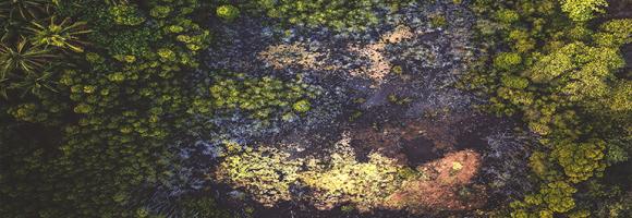
Tropical moist forests have a huge environmental value. They play an important role in biodiversity conservation, terrestrial carbon cycle, hydrological regimes, indigenous population subsistence and human health (1-5). They are increasingly recognized as an essential element of any strategy to mitigate climate change. Deforestation, and degradation compromise the functioning of tropical forests as an ecosystem, lead to biodiversity loss and reduced carbon storage capacity. Deforestation and fragmentation are increasing the risk of virus disease outbreaks. This map shows where deforestation occurred in the last three decades (between 1982 and 2020) and the year when the forest cover has been deforested for the first time (followed or not by a regrowth).
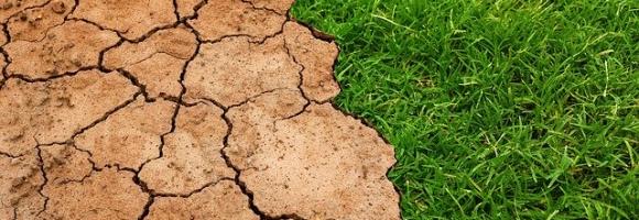
Tropical moist forests have a huge environmental value. They play an important role in biodiversity conservation, terrestrial carbon cycle, hydrological regimes, indigenous population subsistence and human health (1-5). They are increasingly recognized as an essential element of any strategy to mitigate climate change. Deforestation, and degradation compromise the functioning of tropical forests as an ecosystem, lead to biodiversity loss and reduced carbon storage capacity. Deforestation and fragmentation are increasing the risk of virus disease outbreaks. This map shows where degradation occurred in the last three decades (between 1982 and 2020) and the year when the forest has been degraded for the first time (and remained degraded up to 2020).
Côte d'Ivoire and Ghana are the main largest producers of cocoa in the world. However, the cultivation of this crop has led to the loss of vast tracts of forest areas in both countries. Efficient and accurate methods for remotely identifying cocoa farms are essential for the implementation of sustainable cocoa practices and the periodic and effective monitoring of forests. This map, generated using Random Forest image classification, shows the 2019 distribution of cocoa farms in both countries. The estimated area for cocoa is 4.8Mha for Cote d'Ivoire and 2.3Mha for Ghana.
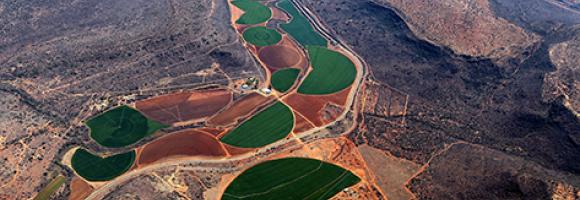
Whether you’re monitoring crops, modelling green energy installations or soil sealing, combatting loss of natural resources or just helping countries meet their Sustainable Development Goals, chances are high that you’ll need an accurate and spatially detailed map on land cover and land use. Earth Observation satellites, like those from EU’s flagship programme Copernicus, are key to providing such maps, at a global scale, with free and open access. Land cover maps represent spatial information on different types (classes) of physical coverage of the Earth's surface, e.g. forests, grasslands, croplands, lakes, wetlands. Dynamic land cover maps include transitions of land cover classes over time and hence captures land cover changes. This dataset shows the land cover for the baseline year 2019 with a discrete classification in 23 classes aligned with UN-FAO's Land Cover Classification System.

From the new available dataset in GFW on tree cover change between 2000 and 2020, here we are displaying the net change in tree cover by percent for country.The net change in tree cover corresponds to the area of gross gain minus the area of gross loss to show the overall change (negative or positive). The attribute table provides also statistics on net change in tree cover such stable forest or disturbed forest(in hectars).
This dataset is accessed through Global Forest Watch on 04/10/2022. www.globalforestwatch.org.
Potapov, P., Hansen, M.C., Pickens, A., Hernandez-Serna, A., Tyukavina, A., Turubanova, S., Zalles, V., Li, X., Khan, A., Stolle, F., Harris, N., Song, X-P., Baggett, A., Kommareddy, I., and Kommareddy, A. 2022. The Global 2000-2020 Land Cover and Land Use Change Dataset Derived From the Landsat Archive: First Results. Frontiers in Remote Sensing, 13, April 2022. https://doi.org/10.3389/frsen.2022.856903; summarized by administrative area at WRI
Tropical moist forests have a huge environmental value. They play an important role in biodiversity conservation, terrestrial carbon cycle, hydrological regimes, indigenous population subsistence and human health (1-5). They are increasingly recognized as an essential element of any strategy to mitigate climate change. Accurate characterization of the tropical moist forests changes is needed to support conservation policies and to better quantify their contribution to global carbon fluxes. The transition map captures the dynamics of changes in tropical moist forests between the initial observation period (1990) and the end of the year 2020.
Tropical moist forests have a huge environmental value. They play an important role in biodiversity conservation, terrestrial carbon cycle, hydrological regimes, indigenous population subsistence and human health (1-5). They are increasingly recognized as an essential element of any strategy to mitigate climate change. Accurate characterization of the tropical moist forests changes is needed to support conservation policies and to better quantify their contribution to global carbon fluxes. This map shows the coverage of undisturbed tropical moist forests remaining at the end of the year 2019.
This dataset compiles geophysical models detailing the thickness of the Earth's outer layers, ranging from surface sedimentary basins down to the base of the lithosphere. The collection serves a dual purpose: it provides broad, global baseline data for sediment distribution, while also offering high-resolution, integrated regional models specifically focused on the African plate.
Dataset Contents:
I. Global Baselines
II. African Regional Models
These layers are part of the Geothermal Atlas for Africa developed within the LEAP-RE project
Forests worldwide are in a state of flux, with accelerating losses in some regions and gains in others. Given the recognized importance of forest ecosystem services, quantification of global forest extent and change is needed. This map displays the tree cover in the year 2000. Tree cover is defined as canopy closure for all vegetation taller than 5m in height and is expressed as a percentage per output grid cell, in the range 0–100.
''Intact Forest Landscapes (IFLs) are defined as those with an unfragmented area of at least 500 km2 and which are minimally influenced by human economic activity''.(Thies et al. 2011) IFLs are critical for stabilizing terrestrial carbon storage, harboring biodiversity, regulating hydrological regimes, and providing other ecosystem functions. Researchers, firstly, created a global IFL map using existing fine-scale maps and
a global coverage of high spatial resolution satellite imagery (Potapov et al. 2008). Moreover they assessed the distribution and dynamics of IFLs within the extent of present-day forest ecosystems tracking loss of intact forest landscapes from 2000 to 2020. In this layer we show the reduction of the IFL extent for African, Caribbean and Pacific (ACP)countries that decreased by 16,6% since the year 2000. Countries that experienced the largest reduction in intact forest landscape area over the past two decades are Solomon Islands with 66,3 %, Central African Republic with 57% and Equatorial Guinea with 50,4%. Democratic Republic of the Congo still has the highest proportion of intactness of ACP countries with 59,7Mha. IFL in Democratic Republic of the Congo has an extent of 64,3Mha as the 27,7% of its forest cover.
| Country | IFL Area in 2000 (sqkm) | IFL Area in 2020 (sqkm) | Percentage of IFL reduction |
| Angola | 2913.32 | 1752.85 | 39.83 |
| Belize | 4275.28 | 3598.44 | 15.83 |
| Cote d'Ivoire | 4558.78 | 3760.48 | 17.51 |
| Cameroon | 52752.96 | 31968.77 | 39.40 |
| Central African Republic | 8695.96 | 3727.14 | 57.14 |
| Congo | 138699.28 | 100215.44 | 27.75 |
| Cuba | 544.02 | 544.02 | 0.00 |
| Democratic Republic of the Congo | 643864.37 | 597275.75 | 7.24 |
| Dominican Republic | 795.21 | 564.89 | 28.96 |
| Equatorial Guinea | 4249.57 | 2104.83 | 50.47 |
| Ethiopia | 3671.63 | 3233.76 | 11.93 |
| Gabon | 108838.30 | 76291.78 | 29.90 |
| Guyana | 144296.97 | 117327.95 | 18.69 |
| Liberia | 4748.74 | 2880.65 | 39.34 |
| Madagascar | 17240.16 | 10799.08 | 37.36 |
| Nigeria | 2959.07 | 2416.10 | 18.35 |
| Papua New Guinea | 159523.52 | 127121.71 | 20.31 |
| Samoa | 650.86 | 643.16 | 1.18 |
| Solomon Islands | 7820.33 | 2630.05 | 66.37 |
| Suriname | 107282.59 | 92574.26 | 13.71 |
| Uganda | 984.66 | 962.06 | 2.30 |
| United Republic of Tanzania | 4081.92 | 3796.32 | 7.00 |
| Vanuatu | 706.13 | 688.33 | 2.52 |

Percentage of cohort of young people three to five years older than the intended age for the last grade of upper secondary level of education who have completed that level of education. This indicator measures the potential impact of electricity on youth education, that represents a crucial pillar for the development of a country.
An intact forest landscape (IFL) is a seamless mosaic of forest and naturally treeless ecosystems with no remotely detected signs of human activity and a minimum area of 500 km2. (Potapov et al.2017) Intact forests are complex and diverse ecosystems that if lost, are irreplaceable. Research shows that designating intact forest landscapes as protected areas has proven effective at limiting their fragmentation. Since 2000, around 100 conserved and protected areas were created in intact forests areas in ACP countries, increasing the percentage of IFL protected from 11% in 2000 to 26% in 2020.
Differences in countries in terms of IFL area reduction: Cuba has not experienced any reduction in IFLs and nowadays its intact forests are fully protected by PAs (544sqkm). At the contrary Angola still not has any kind of protection for its IFLs and experienced a reduction of 39,83% of its IFL (1160 sqkm) in country.The reduction of IFL area in ACP countries was higher outside PAs (19%) than within PAs (5%).Madagascar is the country where the reduction of IFL areas was very high inside protected areas (2420 sqkm). The IFL loss inside PAs has been more than 40% between 2000 and 2020. Central African Republic experienced 23% of reduction inside PAs (938,13 sqkm). This layer shows the percentage of IFLs protected by country
| Country | IFL protected 2020 (sqkm) | IFL unprotected 2020 (sqkm) | Percentage of IFL protected 2020 | Percentage of IFL unprotected 2020 |
| Angola | 0.00 | 1752.85 | 0.00 | 100.00 |
| Belize | 3310.17 | 288.36 | 91.99 | 8.01 |
| Cameroon | 19181.16 | 12787.52 | 60.00 | 40.00 |
| Central African Republic | 3070.21 | 656.90 | 82.37 | 17.62 |
| Congo | 67218.88 | 32997.23 | 67.07 | 32.93 |
| Cote d'Ivoire | 3759.21 | 1.27 | 99.97 | 0.03 |
| Cuba | 544.02 | 0.00 | 100.00 | 0.00 |
| Democratic Republic of the Congo | 131588.22 | 465687.18 | 22.03 | 77.97 |
| Dominican Republic | 553.86 | 11.03 | 98.05 | 1.95 |
| Equatorial Guinea | 1549.39 | 555.44 | 73.61 | 26.39 |
| Ethiopia | 0 | 3233.7 | 0 | 100 |
| Gabon | 22692.90 | 53598.80 | 29.74 | 70.26 |
| Guyana | 15545.93 | 101781.93 | 13.25 | 86.75 |
| Liberia | 1573.69 | 1306.95 | 54.63 | 45.37 |
| Madagascar | 9931.34 | 867.74 | 91.96 | 8.04 |
| Nigeria | 2211.75 | 204.39 | 91.54 | 8.46 |
| Papua New Guinea | 5863.48 | 121258.17 | 4.61 | 95.39 |
| Samoa | 93.13 | 550.03 | 14.48 | 85.52 |
| Solomon Islands | 60.11 | 2569.93 | 2.29 | 97.71 |
| Suriname | 17304.85 | 75269.36 | 18.69 | 81.31 |
| Uganda | 945.21 | 16.84 | 98.25 | 1.75 |
| United Republic of Tanzania | 3627.46 | 168.85 | 95.55 | 4.45 |
| Vanuatu | 13.24 | 675.08 | 1.92 | 98.08 |
Analysis performed by Simona Lippi
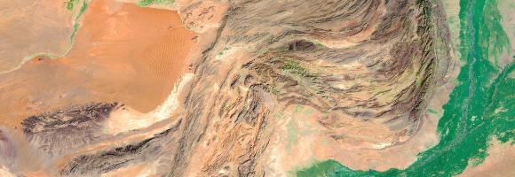
At any given place on Earth, complex human-environment interactions are at play. They include differing rates and magnitudes of drivers (e.g. overgrazing, climate change, agricultural practices) and differing consequences in land degradation (e.g. soil erosion, changes in productivity, loss of biodiversity). The occurrence of multiple global change issues at a location suggests a potential for land degradation, at least in some form. This layer depicts where global change issues relevant to land degradation coincide at a global scale. It helps identifying local or regional areas of concern where land degradation processes may be underway.
Park managers in many countries across Africa need to monitor and understand their parks features and overall health. They can rely on the highly detailed land cover information offered by the Copernicus Hot Spot Land Cover Change Explorer for specific areas of interest –or hot spots. These areas were selected for their importance in biodiversity preservation (Protected Areas, Key Landscapes for Conservation...). For each land cover class (Natural vegetation, Wetlands, urbane areas, etc.), this layer shows which portions of the areas changed to another class over the period (2000-2019). For a more detailed analysis, compare the layer with the present landcover or refer to the online Explorer. The allows to monitor land cover and land cover change in high detail and make informed decisions based on spatial data.
Copernicus is the European flagship programme for monitoring the Earth. Data is collected by Earth observation satellites and sensors on the earth’s surface. The Copernicus Land Monitoring Service provides geographical information on land use and land cover at European and global scale. Derived from the Copernicus Hot Spot Land Cover Change Explorer, this layer presents detailed land cover information for specific areas of interest –or hot spots– in Africa. These areas were selected as a priority for mapping because of their importance in biodiversity preservation (Protected Areas, Key Landscapes for Conservation...). Park managers in many countries across Africa rely on this Copernicus product to monitor and understand their parks features and overall health. Mapping habitats, assessing pressure on land, identifying prime locations for species reintroduction or new areas to protect are just a few examples of how these data can be exploited.
Crop conditions monitoring is highly relevant for food security early warning and response planning in food-insecure areas of the world. GEOGLAM (the Group on Earth Observations' Global Agricultural Monitoring Initiative) aims to reinforce the international community's capacity to produce and disseminate relevant, timely, and accurate forecasts of agricultural production at national, regional, and global scales using Earth Observation data.
Copernicus4GEOGLAM, one of the Copernicus Land Monitoring Services managed by the EC Joint Research Centre, aims to produce baseline information that allows countries in Africa to improve their agricultural monitoring systems.
This dataset aggregates crop maps requested by three East African nations, showing the agricultural situation at the end of the long rain season of 2021. The results are made fully and freely accessible, covering the following areas:
This dataset provides a continent-wide, raster-based spatial representation of Earth's surface heat flow across the African tectonic plate for the year 2013, modeled under a historical baseline scenario. The data quantifies the amount of thermal energy moving from the Earth's interior to its surface, with values explicitly expressed in watts per square meter (W/m²). This resource is critical for identifying geothermal potential, understanding tectonic anomalies, and supporting broader geoscientific and energy research.
Sources and ContextThis layer is part of the Geothermal Atlas for Africa developed within the LEAP-RE project

Percentage of children aged 6-8 that currently attends, or in the current school year attended, school. This indicator measures the potential educational impact of bringing electricity to schools; therefore, the impact of binging electricity will be higher where the educational attendance is low.
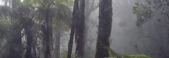
Forest canopy height measures the average height of the tree canopy in 2012. This dataset is created by integrating broadscale optical remotely sensed data at 30-metre spatial resolution with on-the-ground measurements.
The GHS-BUILT-S spatial raster dataset depicts the distribution of the built-up (BU) surfaces estimates between 1975 and 2030 in 5 year intervals and two functional use components a) the total BU surface and b) the non-residential (NRES) BU surface. The data is made by spatial-temporal interpolation of five observed collections of multiple-sensor, multiple-platform satellite imageries: Landsat (MSS, TM, ETM sensor) data supports the 1975, 1990, 2000, and 2014 epochs, while a Sentinel-2 (S2) image composite (GHS-composite-S2 R2020A) supports the 2018 epoch.
This data represents the total BU surface (square meters) for year 2020 over cells of 1x1 km size.
The GHS-BUILT-S spatial raster dataset depicts the distribution of the built-up (BU) surfaces estimates between 1975 and 2030 in 5 year intervals and two functional use components a) the total BU surface and b) the non-residential (NRES) BU surface. The data is made by spatial-temporal interpolation of five observed collections of multiple-sensor, multiple-platform satellite imageries: Landsat (MSS, TM, ETM sensor) data supports the 1975, 1990, 2000, and 2014 epochs, while a Sentinel-2 (S2) image composite (GHS-composite-S2 R2020A) supports the 2018 epoch.
This data represents the total BU surface estimates (square meters) for year 2020 over cells of 100x100 m size.
This data represents the total built-up volume between 1975 and 2030 in 5 year intervals over cells of 1x1 km size.
It derives from the GHS-BUILT-V - R2023A spatial raster dataset, that depicts the distribution of built-up volumes, expressed as number of cubic metres. The data report about the total built-up volume and the built-up volume allocated to dominant non-residential (NRES) uses.
The dataset is part the Global Human Settlement Layer , Global, high-resolution, multi-temporal gridded data on built-up environment (built-up surface, built-up volume, residential vs. non-residential function), resident population, and settlement classification by the UN-recommended methodology “degree of urbanisation”. The complete information about the GHSL main products can be found in the GHSL Data Package 2023 report
This data represents the distribution of human population between 1975 and 2030 in 5 year intervals over cells of 1x1 km size.
It derives from the GHS-POP - R2023A. Residential population estimates between 1975 and 2020 in 5-year intervals and projections to 2025 and 2030 derived from CIESIN GPWv4.11 were disaggregated from census or administrative units to grid cells, informed by the distribution, volume, and classification of built-up as mapped in the Global Human Settlement Layer (GHSL) global layer per corresponding epoch.
The dataset is part the Global Human Settlement Layer, that provide global, high-resolution, multi-temporal gridded data on built-up environment (built-up surface, built-up volume, residential vs. non-residential function), resident population, and settlement classification by the UN-recommended methodology “degree of urbanisation”. The complete information about the GHSL main products can be found in the GHSL Data Package 2023 report.

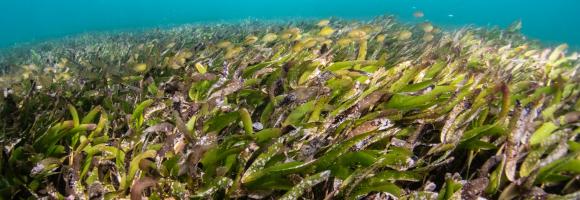
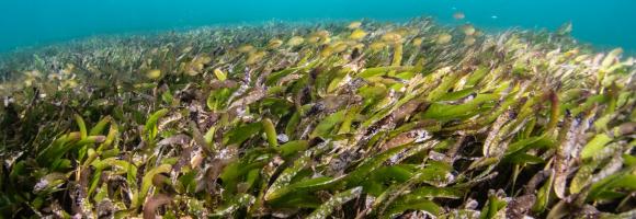
Seagrass is found on all continents except Antarctica, covering roughly 0.1% of the ocean floor. However, its global extent remains inadequately mapped, with estimates varying between 160,387 km² and 670,000 km², posing a significant challenge for conservation efforts. The UNEP-WCMC seagrass dataset indicates that Africa harbors approximately 12% of the world’s seagrass.
Seagrass is found on all continents except Antarctica, covering roughly 0.1% of the ocean floor. However, its global extent remains inadequately mapped, with estimates varying between 160,387 km² and 670,000 km², posing a significant challenge for conservation efforts. The UNEP-WCMC seagrass dataset indicates that Africa harbors approximately 12% of the world’s seagrass.
The Global Gridded Relative Deprivation Index (GRDI) characterizes the relative levels of multidimensional deprivation and poverty, where a value of 100 represents the highest level of deprivation and a value of 0 the lowest. GRDI is built from sociodemographic and satellite data inputs that were spatially harmonized, indexed, and weighted into six main components to produce the final GRDI layer.
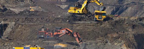
Mining has major economic, environmental and societal consequences, yet knowledge and understanding of its global footprint are still limited. These polygons represent the global mining land use detected via remote sensing analysis of high-resolution, publicly available satellite imagery. The dataset comprises 74,548 polygons, covering ~66,000 km2 of features like waste rock dumps, pits, water ponds, tailings dams, heap leach pads and processing/milling infrastructure.
In 2020, a group of researchers carried out analysis to examine the importance of Indigenous Peoples’ lands for preserving Intact Forest Landscapes.(Fa et al.2020)They used geospatial data on the extent of Indigenous Peoples’ lands reported by Garnett et al. (2018), and Geospatial data for IFLs were sourced from the Intact Forest Landscapes website (www.intactforests.org) for the years 2000, 2013, and 2016 (Potapov et al. 2017)In the paper they have shown that the proportion of Indigenous Peoples’ lands mapped as IFLs was considerably higher (10.9%) than the proportion of other lands (defined here as all land outside Indigenous Peoples’ lands) mapped as IFLs (6.8%).
In this map we reported the percentage of Intact Forest Lansdcapes reduction in Indigenous People Lands for the period 2000-2016. IN the table we reported also the percentage of IFLs reduction in other lands. To explore more IFLs conservation strategies for African, Caribbean and Pacific countries you can check BIOPAMA Geonode Layers
Sources:
Fa JE, Watson JE, Leiper I, Potapov P, Evans TD, Burgess ND, Molnár Z, Fernández‐Llamazares Á, Duncan T, Wang S, Austin BJ. Importance of Indigenous Peoples’ lands for the conservation of Intact Forest Landscapes. Frontiers in Ecology and the Environment. 2020 Apr;18(3):135-4
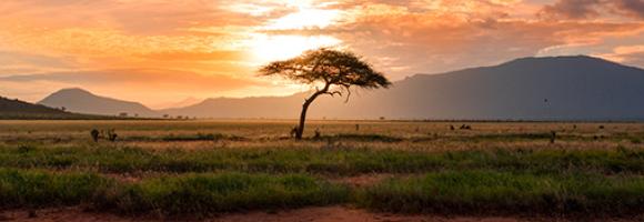
Some areas in Africa represent spectacular, still viable examples of Africa’s wildlife and wild places. They are of such outstanding importance and value that they should be conserved at all costs and in principle forever. Those areas are referred to as Key Landscapes for Conservation or KLCs. A suitable network of KLCs has the potential to protect the well-known wildlife species within natural ecosystems and to stimulate rural economic growth.
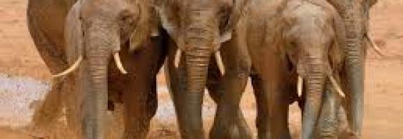
<p>This spatial dataset contains the geographic boundaries and ecological evaluations of 45 Key Landscapes for Conservation and Development (KLCDs) across Sub-Saharan Africa. Building on the <a href="https://africa-knowledge-platform.ec.europa.eu/dataset/key-landscapes-c…; Key Landscapes for Conservation (KLCs) </a> identified in the EU report <a href="https://op.europa.eu/sl/publication-detail/-/publication/d76ac7eb-bc4a-…;“Larger than elephants”</a>, the NaturAfrica initiative is rolled out across these key biodiversity and development landscapes.</p>
<p>NaturAfrica's efforts are concentrated on ‘mega-landscapes’—biogeographical regions identified as crucial for both conservation and development. These regions encompass:</p>
<ul>
<li>The forest ecosystems of the Congo Basin;</li>
<li>Landscapes of transhumance pastoralists in North Cameroon, the Central African Republic, and Chad;</li>
<li>Guinean forests of West Africa;</li>
<li>Savannahs in the Sudano-Sahelian zone of West Africa;</li>
<li>Savannahs and watersheds of the East Africa rift;</li>
<li>Transfrontier conservation areas of Southern Africa.</li>
</ul>
<p>The layer was developed to support the prioritization of intervention areas for the second phase of this initiative, which combines conservation with sustainable job creation. It provides a spatially explicit characterization of ecological value across these landscapes, evaluated and attributed based on five core ecological and environmental dimensions:</p>
<ul>
<li><span class="label">Threatened Species Richness:</span> Concentration and diversity of threatened species.</li>
<li><span class="label">Species Endemicity:</span> Presence of endemic species unique to the specific geographic region.</li>
<li><span class="label">Ecosystem Integrity:</span> The integrity of protected and conserved areas, accounting for degrees of human modification and habitat fragmentation.</li>
<li><span class="label">Ecological Connectivity:</span> The degree of connectivity and spatial linkages between protected and conserved areas.</li>
<li><span class="label">Ecosystem Services:</span> Provisioning and regulating services, with a specific focus on carbon storage and water services.</li>
</ul>
<strong>Purpose</strong>
<p>The layer was created to inform the EC Directorate General for International Partnerships (DG INTPA) and policymakers in selecting and prioritizing funding intervention areas based on specific targets (e.g., species conservation, connectivity, or water security) within different biogeographical regions. It serves as a spatial decision-support tool to align with the European Green Deal and the EU Biodiversity Strategy for 2030.</p>
<strong>Geographic Extent</strong>
<ul>
<li><span class="label">Region:</span> Sub-Saharan Africa</li>
<li><span class="label">Coverage:</span> 45 distinct Key Landscapes for Conservation and Development (KLCDs)</li>
</ul>
<strong>Keywords</strong>
<ul>
<li><span class="label">Thematic:</span> Biodiversity Conservation, NaturAfrica, Ecosystem Services, Protected Areas, Habitat Connectivity, Species Endemicity, European Green Deal, Ecosystem Integrity, Transfrontier Conservation, Mega-landscapes.</li>
<li><span class="label">Spatial:</span> Sub-Saharan Africa, Congo Basin, West Africa, East Africa, Southern Africa, Sudano-Sahelian zone.</li>
</ul>
<strong>Lineage / Data Source</strong>
<p>This dataset is derived from the <a href="https://publications.jrc.ec.europa.eu/repository/handle/JRC145021"> technical assessment conducted for the European Commission Knowledge Centre for Biodiversity (KCBD) </a>.</p>
Land cover is defined as the physical material at the surface of the earth, usually documented via the interpretation of earth observations. Common land cover types include trees, grass, bare ground, built up areas, water, etc. How well are different ecosystem types (as indicated by land cover) preserved and how strong are anthropogenic changes affecting their distribution in a given area? Human pressures are constantly increasing and it is important to monitor the consequences of the associated changes on the environment. This map shows the changes in land cover between 1995 and 2015.

This layer provides estimates of the percentage of children aged 2 to 10 years (PfPR2–10) with detectable Plasmodium falciparum parasites in 2022. The estimates are generated using geostatistical models based on point prevalence surveys, routine surveillance data, and a wide range of geospatial covariates representing mosquito habitat and environmental conditions. The data are available annually from 2000 onward, covering all malaria-endemic countries, at a spatial resolution of 5 × 5 km.
The map is based on Copernicus Global Land Cover data which shows actual land cover (what physically covers land across the globe—forests, grasslands, croplands, lakes, wetlands, built-up area, etc) at 100m x 100m resolution. The land cover data for Africa was overlaid on (high resolution) satellite imagery of Africa, which is then used to determine the land use (by visual interpretation) associated with the various land cover patterns on the Copernicus Global Land Cover map.
Copernicus land cover data offers several advantages: it is of high quality, has a high resolution (100m x 100m), and offers time series satellite imagery. More importantly, the Copernicus Global Land Service is a continuous process and its datasets are updated annually. This means that the Soils4Africa map of agricultural land can be updated every time the land cover data for the new year becomes available (the map is currently based on 2019 data).
The Copernicus dataset already includes the category ‘cropland,’ which by definition is part of agricultural land. The Soils4Africa map broadens the scope of that dataset by infering information on agricultural use and including other kinds of agricultural land use such as grazing pastures and plantations.
When land is mapped as other than ‘cropland'-- like ‘shrubland’ for example-- it is more difficult to interpret and determine whether it is under agricultural use. The Copernicus dataset includes information about ‘fractional cover’-- or the percentage of a particular pixel under a particular kind of land cover (for example, 30% of a 100m x 100m pixel could be forest and 20% could be shrubland). The Soils4Africa map takes into account how fractional cover varies over an area to establish rules for interpreting its land cover data to determine whether it is under agricultural use and for what purpose. These rules were validated by comparing it with ground level information on land use (or land use pattern) for specific areas drawn from the interpretation of satellite imagery from Google Earth.
For example, ground-level observation shows that forest cover upwards of 30% in a given area when matched by shrubland cover of over 30%, is characterized by woody vegetation with a smooth canopy. Therefore, such area is more likely to be under plantations rather than natural forest. Thus, such an area should be counted as agricultural land, even if less than 15% of it is under crops.
Substantial crop losses occur at various stages along the postharvest value chain. Losses result from poor handling and storage practices combined with limited awareness, infrastructure, and knowledge. The African Postharvest Losses Information System (APHLIS) (www.aphlis.net) is the foremost international effort to collect, analyse and disseminate data on postharvest losses of cereal grains in sub-Saharan Africa. The cumulative % loss in weight incurred during harvesting, drying, threshing/shelling, winnowing, household-level storage, transport and market-level storage for the selected crop, location, and year is presented. Complimentary data sets are collected and used to convert this % loss into absolute loss values in tonnes, US$ and nutrients, along with the nutritional and financial impacts of these losses by province and country. Understanding the magnitude of postharvest loss, the points in the value chain where losses occur, and the causes and impacts of loss helps decision-makers formulate effective policies and invest in successful postharvest loss programmes.
Substantial crop losses occur at various stages along the postharvest value chain. Losses result from poor handling and storage practices combined with limited awareness, infrastructure, and knowledge. The African Postharvest Losses Information System (APHLIS) (www.aphlis.net) is the foremost international effort to collect, analyse and disseminate data on postharvest losses of cereal grains in sub-Saharan Africa. The cumulative % loss in weight incurred during harvesting, drying, threshing/shelling, winnowing, household-level storage, transport and market-level storage for the selected crop, location, and year is presented. Complimentary data sets are collected and used to convert this % loss into absolute loss values in tonnes, US$ and nutrients, along with the nutritional and financial impacts of these losses by province and country. Understanding the magnitude of postharvest loss, the points in the value chain where losses occur, and the causes and impacts of loss helps decision-makers formulate effective policies and invest in successful postharvest loss programmes.
Substantial crop losses occur at various stages along the postharvest value chain. Losses result from poor handling and storage practices combined with limited awareness, infrastructure, and knowledge. The African Postharvest Losses Information System (APHLIS) (www.aphlis.net) is the foremost international effort to collect, analyse and disseminate data on postharvest losses of cereal grains in sub-Saharan Africa. The cumulative % loss in weight incurred during harvesting, drying, threshing/shelling, winnowing, household-level storage, transport and market-level storage for the selected crop, location, and year is presented. Complimentary data sets are collected and used to convert this % loss into absolute loss values in tonnes, US$ and nutrients, along with the nutritional and financial impacts of these losses by province and country. Understanding the magnitude of postharvest loss, the points in the value chain where losses occur, and the causes and impacts of loss helps decision-makers formulate effective policies and invest in successful postharvest loss programmes.
Substantial crop losses occur at various stages along the postharvest value chain. Losses result from poor handling and storage practices combined with limited awareness, infrastructure, and knowledge. The African Postharvest Losses Information System (APHLIS) (www.aphlis.net) is the foremost international effort to collect, analyse and disseminate data on postharvest losses of cereal grains in sub-Saharan Africa. The cumulative % loss in weight incurred during harvesting, drying, threshing/shelling, winnowing, household-level storage, transport and market-level storage for the selected crop, location, and year is presented. Complimentary data sets are collected and used to convert this % loss into absolute loss values in tonnes, US$ and nutrients, along with the nutritional and financial impacts of these losses by province and country. Understanding the magnitude of postharvest loss, the points in the value chain where losses occur, and the causes and impacts of loss helps decision-makers formulate effective policies and invest in successful postharvest loss programmes.
Substantial crop losses occur at various stages along the postharvest value chain. Losses result from poor handling and storage practices combined with limited awareness, infrastructure, and knowledge. The African Postharvest Losses Information System (APHLIS) (www.aphlis.net) is the foremost international effort to collect, analyse and disseminate data on postharvest losses of cereal grains in sub-Saharan Africa. The cumulative % loss in weight incurred during harvesting, drying, threshing/shelling, winnowing, household-level storage, transport and market-level storage for the selected crop, location, and year is presented. Complimentary data sets are collected and used to convert this % loss into absolute loss values in tonnes, US$ and nutrients, along with the nutritional and financial impacts of these losses by province and country. Understanding the magnitude of postharvest loss, the points in the value chain where losses occur, and the causes and impacts of loss helps decision-makers formulate effective policies and invest in successful postharvest loss programmes.
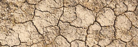
Droughts affect millions of people in the world each year and have long-lasting socioeconomic impacts. They can occur over most parts of the world, even in wet and humid regions, and can profoundly impact agriculture, basic household welfare, tourism, ecosystems and the services they provide. The Risk of Drought Impact for Agriculture (RDrI-Agri) is a categorized risk index, indicating the probability of having impacts from a drought, with particular focus on vegetation. Higher risk (in red) means that the areas affected will be the most likely to report impacts due to droughts. It is updated every ten days.
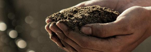
In most people's mind, soil would not figure highly in a list of the natural resources of Africa. However, healthy and fertile soils are the cornerstones of food security, key environmental services, social cohesion and the economies of most African countries. Unfortunately, soil in Africa tends to reach public awareness only when it fails – often with catastrophic consequences as seen by the famine episodes of the Sahel in the 1980s and more recently in Niger and the Horn of Africa. In the context of major global environmental challenges such as food security, climate change, fresh water scarcity and biodiversity loss, the protection and the sustainable management of soil resources in Africa are of paramount importance. This layer presents the diversity of soil types across Africa. This map was produced by the Joint Research Centre of the European Commission for the Soil Atlas of Africa.
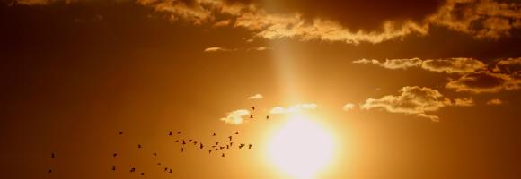
African countries have an evident potential for solar energy. Knowing the amount of solar radiation reaching the earth's surface is of particular interest for photovoltaic installations. It can be represented by the Global Horizontal Irradiation: the total amount of energy received from the Sun by a surface horizontal to the ground during a period of time, expressed in Wh/m2. This map shows the yearly average (2005-2015) global horizontal irradiation (kWh/m2).
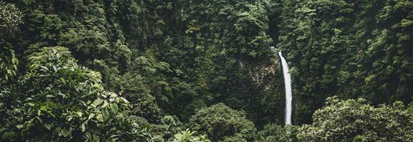
Forests worldwide are in a state of flux, with accelerating losses in some regions and gains in others. Given the recognized importance of forest ecosystem services, quantification of global forest extent and change is needed. This map displays the forest gain during the period 2000–2018. Forest gain is defined as the inverse of loss, or a change from non-forest to forest entirely within the study period. It is expressed as either 1 (gain) or 0 (no gain).
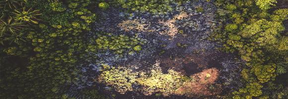
Forests worldwide are in a state of flux, with accelerating losses in some regions and gains in others. Given the recognized importance of forest ecosystem services, quantification of global forest extent and change is needed. This map displays the forest loss during the period 2000–2018, defined as a stand-replacement disturbance, or a change from forest to non-forest state. It is expressed as either 1 (loss - in red) or 0 (no loss).
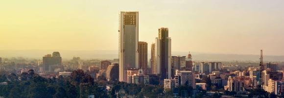
This data represents the total built-up volume between 1975 and 2030 in 5 year intervals over cells of 1x1 km size.
It derives from the GHS-BUILT-V - R2023A spatial raster dataset, that depicts the distribution of built-up volumes, expressed as number of cubic metres. The data report about the total built-up volume and the built-up volume allocated to dominant non-residential (NRES) uses.
The dataset is part the Global Human Settlement Layer , Global, high-resolution, multi-temporal gridded data on built-up environment (built-up surface, built-up volume, residential vs. non-residential function), resident population, and settlement classification by the UN-recommended methodology “degree of urbanisation”. The complete information about the GHSL main products can be found in the GHSL Data Package 2023 report
This data represents the distribution of human population between 1975 and 2030 in 5 year intervals over cells of 1x1 km size.
It derives from the GHS-POP - R2023A. Residential population estimates between 1975 and 2020 in 5-year intervals and projections to 2025 and 2030 derived from CIESIN GPWv4.11 were disaggregated from census or administrative units to grid cells, informed by the distribution, volume, and classification of built-up as mapped in the Global Human Settlement Layer (GHSL) global layer per corresponding epoch.
The dataset is part the Global Human Settlement Layer, that provide global, high-resolution, multi-temporal gridded data on built-up environment (built-up surface, built-up volume, residential vs. non-residential function), resident population, and settlement classification by the UN-recommended methodology “degree of urbanisation”. The complete information about the GHSL main products can be found in the GHSL Data Package 2023 report.
This data represents the distribution of human population between 1975 and 2030 in 5 year intervals over cells of 100x100 m size.
It derives from the GHS-POP - R2023A. Residential population estimates between 1975 and 2020 in 5-year intervals and projections to 2025 and 2030 derived from CIESIN GPWv4.11 were disaggregated from census or administrative units to grid cells, informed by the distribution, volume, and classification of built-up as mapped in the Global Human Settlement Layer (GHSL) global layer per corresponding epoch.
The dataset is part the Global Human Settlement Layer, that provide global, high-resolution, multi-temporal gridded data on built-up environment (built-up surface, built-up volume, residential vs. non-residential function), resident population, and settlement classification by the UN-recommended methodology “degree of urbanisation”. The complete information about the GHSL main products can be found in the GHSL Data Package 2023 report.
These layers present the application of the Degree of Urbanisation stage I methodology recommended by UN Statistical Commission to the global population grid generated by the JRC in the epochs 1975-2030 (5 years timestep).
They derive from the GHS-SMOD - R2023A.
The layers have been generated by integration of built-up surface extracted from Landsat and Sentinel-2 image data processing (GHS-BUILT-S R2023), and population data derived from the CIESIN GPW v4.11 (GHS-POP R2023).
The dataset is part the Global Human Settlement Layer, that provide global, high-resolution, multi-temporal gridded data on built-up environment (built-up surface, built-up volume, residential vs. non-residential function), resident population, and settlement classification by the UN-recommended methodology “degree of urbanisation”. The complete information about the GHSL main products can be found in the GHSL Data Package 2023 report.
The current version of the GDW database (version 1.0) aims to catalogue all types of anthropogenic instream barriers. While initial mapping efforts prioritize major dams that form reservoirs, as well as run-of-river barriers on larger rivers where more information is readily available, the dataset comprises two distinct but interconnected spatial layers: