Main navigation
User account menu
Language

Higher energy demands in Africa has led to a wide expansion of the number of hydropower sites, mainly between the 1960s and 1980s. The construction of dams causes impoundments of rivers and reservoirs in the regions of dam influence, with higher evaporation and water temperatures due to increased water surfaces. This map shows the he surface area (sqkm) of African reservoirs subject to hydropower production for the year 2016. It includes reservoirs of associated hydropower plants with installed capacities above 5MW. Apart from this, only reservoirs with a detected dam-caused impoundment of water surface are considered.
The hydropower installed capacity indicates the amount of energy a hydropower plant can produce in its turbines. In 2016, hydropower accounted for 54% of the installed capacity in Eastern Africa, 58% in Central Africa and 30% in Western Africa with fourteen countries having a hydropower share above 50% and eight countries above 70%. These highly hydropower-dependent countries are particularly prone to electricity cuts due to the lack of water caused by severe droughts. This map shows the location and installed capacities of hydropower plants above 5MW installed capacity in Africa for year 2016, representing 95% of the total hydropower installed capacity in Africa.
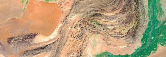
Some extraordinary changes have occurred across the globe over the past decades regarding human habitation. Globally, between 1975 and 2015 built-up areas increased by approximately 250 %, while population increased by a factor of 1.8. The most considerable changes occurred in Africa where it has nearly quadrupled. The extent of built-up area poses a number of challenges to global sustainable development. As urban clusters expand, productive land and soil is sealed, and natural ecosystems are replaced by land use to support urban centres. This layer highlights the areas of concern for built-up related issues derived from the convergence of global evidence of human-environment interactions that can have land degradation consequences.
Many African countries, especially in the Sub-Saharan region highly depend on hydropower which is one of the energy sources that are most affected by droughts. At the same time hydropower has a huge impact on water consumption (mainly through evaporation from reservoir surfaces) in comparison with other fuel types despite having higher densities of plants and installed capacities. Hydropower accounts for 15% of Africa’s energy production. This map shows the energy production (GWh) of hydropower plants with an installed capacity above 5MW, aggregated for each hydropower-generating country in Africa for year 2016.

African countries have an evident potential for solar energy. Knowing what amount of solar radiation reaches the earth's surface is of particular interest for solar photovoltaic (PV) installations. It can be represented by the average annual potential energy production (or yield): the total amount of electricity (kWh) produced in one year by a 1 kWp PV system at optimal angle, expressed in kWh/kWp.

Increasing water scarcity and water quality issues are serious constraints, especially for Northern Africa. A comprehensive assessment of spatial and temporal precipitation frequency is the initial step for defining public policies relating to water resources management and environmental monitoring. In the agricultural sector, a detailed knowledge of precipitation patterns is necessary to identify the most appropriate crop varieties for the region and to effectively manage climate related uncertainties. Precipitation frequency is also a central source of information for hazard mitigation and management. This layer represents the average variability of precipitation (L-CV) around the annual mean value for the period 1981-2017. The larger the L-CV, the more variable the annual precipitation is from year to year.
Aridity represents the ‘dryness’ of the climate. Dry areas have a higher potential for land degradation. This layer displays the areas of concern for aridity related issues derived from the convergence of global evidence of human-environment interactions that can lead to land degradation. It highlights dryland areas, where the Aridity Index (ratio of precipitation to evapotranspiration) is inferior to 0.65.
This layer is part of the World Altas of Desertification
Increasing water scarcity and water quality issues are serious constraints, especially for Northern Africa. A comprehensive assessment of spatial and temporal precipitation frequency is the initial step for defining public policies relating to water resources management and environmental monitoring. In the agricultural sector, a detailed knowledge of precipitation patterns is necessary to identify the most appropriate crop varieties for the region and to effectively manage climate related uncertainties. Precipitation frequency is also a central source of information for hazard mitigation and management. This layer shows the average annual precipitation (mm/year) for the period 1981-2017 across the continent.

Map showing the average continental surface temperature of the year 2022. This map was created by interpolating raw monthly satellite data to fill holes in the grids and subsequently adding and averaging the monthly surface temperatures of the year 2022. The data is clipped to only show the African continental region. The raw data is collected during the daytime by the Moderate Resolution Imaging Spectroradiometer (MODIS), an instrument on NASA's Terra and Aqua satellites. Please note that the type of "surface" MODIS measures varies as a function of location. In some places, the measurement represents the skin temperature of the bare land surface. In other places, the temperature represents the skin temperature of whatever is on the land-including snow and ice, or the leafy canopy of forests and crop fields, or human-made structures such as pavement and building rooftops.
Values are expressed in °C.
This dataset is part of the LEAP-RE project collection. For more information visit https://www.leap-re.eu/

The Copernicus Global Land Service - Burnt Area products depict burn scars, surfaces which have been sufficiently affected by fire to display significant changes in the vegetation cover (destruction of dry material, reduction or loss of green material) and in the ground surface (temporarily darker because of ash). The monthly products are available at global scale in the spatial resolution of 300 m and cover the period from January 2019 to April 2022. The pixel bears the value of the day of the year in which the burn scars were visible while, if selected for mapping in this platform, the dataset shows the burn scars detected in the selected month.
Changes in vegetation biomass are critical in assessing land degradation. Climate variations, alone or in combination with human-induced land use and land change, can affect biomass productivity and may trigger changes in vegetation type and structure. Depending on their severity and duration, precipitation anomalies can trigger or aggravate existing land pressures. This layer displays the areas of concern for climate-vegetation trends derived from the convergence of global evidence of human-environment interactions that can have consequences on land degradation. It highlights areas with declining plant productivity in response to climate fluctuations (drought conditions in particular).

Healthy coral reefs provide a home for millions of aquatic species and numerous ecosystemic services. Yet they are severely threatened. When stressed, corals expel the symbiotic algae living in their tissues and become white (bleached) and vulnerable. The NOAA Coral Reef Watch daily global 5km satellite coral Bleaching Alert Area (7-day maximum) is a composite product that summarizes the current Degree Heating Week (a cumulative measurement of both intensity and duration of heat stress) and Coral Bleaching HotSpot (occurrence and magnitude of instantaneous heat stress) values. At a glance, this layer outlines the current locations, coverage, and potential risk level of coral bleaching heat stress.
Humans need increasingly more biomass for food, fodder, fibre and energy. Meeting these demands changes global ecosystems. Tracking changes in total biomass production or land productivity is an essential part of monitoring land transformations that are typically associated with land degradation. Land productivity dynamics (LPD) are used as an indicator of change or stability of the land’s capacity to sustain primary production. This layer displays the areas of concern for land productivity related issues, derived from the convergence of global evidence of human-environment interactions that can have consequences on land degradation.
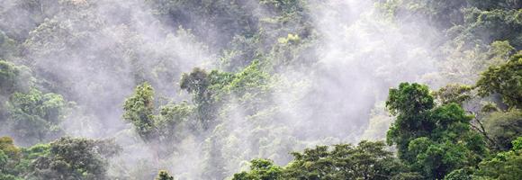
This layer provides the Effective Leaf Area Index (LAIe), a critical parameter for modeling evapotranspiration and carbon fluxes between the biosphere and the atmosphere. Monitoring the distribution and seasonal evolution of LAI is essential for assessing vegetation health and ecosystem dynamics across Africa.
The Effective Leaf Area Index is a quantitative measure of the amount of live green leaf material present per unit ground surface. Unlike "True LAI," which represents the total physical leaf area, the Effective LAI is derived from canopy gap fraction measurements and assumes a random distribution of foliage. It is a non-dimensional quantity, typically expressed in units of m²/m².
This dataset is widely utilized in agro-meteorology, biogeochemical modeling, and General Circulation Models (GCMs) to parameterize vegetation cover and its complex interactions with the atmosphere.
This layer is part of the Earth Land Information System (ELIS).
This layer presents the Effective Leaf Area Index (LAIe) Anomalies, representing the deviation of current vegetation density from the historical average. Monitoring the change of LAI is essential for assessing the evolution of the vegetation over Africa.
LAI anomalies are calculated relative to the average values between 2003 and 2010. The dataset captures LAI anomalies every 10 days, reflecting the high variability and rapid changes in African vegetation cover. Increases in temperature and precipitation deficits are the primary drivers for negative anomalies (reduced foliage density). Beyond climatic factors, human activities or animal grazing may also locally impact the state and density of leaves.
This layer is part of the a href="https://fapar.jrc.ec.europa.eu/_www/index.php">Earth Land Information System (ELIS).

Displays areas where the geographic range of two or more endemic bird species overlaps. While many bird species are widespread, over 2,500 are endemic and restricted to an area smaller than 5 million hectares (restricted-range species). BirdLife International has mapped every restricted-range species using geo-referenced locality records. Through this process, they identified regions of the world—known as “Endemic Bird Areas” (EBAs)—where the distributions of two or more of these species overlap. Half of all restricted-range species are globally threatened or near-threatened, and the other half remain vulnerable to loss or degradation of habitat. The majority of EBAs are also important for the conservation of restricted-range species from other animal and plant groups. The unique landscapes where these bird species occur, amounting to just 4.5% of the earth's land surface, are high priorities for broad-scale ecosystem conservation. Geographically, EBAs are often islands or mountain ranges, and vary considerably in size, from a few hundred hectares to more than 10,000,000 hectares. EBAs also vary in the number of restricted-range species that they support (from two to 80). EBAs are found around the world, but most (77%) of them are located in the tropics and subtropics.
Fire is a natural part of all ecosystems. Wildfires have been burning vegetation and shaping landscapes far longer than people have been on Earth. However, changes in fire frequency and timing can result in degradation if the vegetation is not adapted to the new fire regimes. This can cause long-term damage to land biomass components affecting soil structure, nutrients and water cycling. This layer displays the areas of concern for fires related issues derived from the convergence of global evidence of human-environment interactions that can have consequences on land degradation.

The GHS-BUILT-S spatial raster dataset depicts the distribution of the built-up (BU) surfaces estimates between 1975 and 2030 in 5 year intervals and two functional use components a) the total BU surface and b) the non-residential (NRES) BU surface. The data is made by spatial-temporal interpolation of five observed collections of multiple-sensor, multiple-platform satellite imageries: Landsat (MSS, TM, ETM sensor) data supports the 1975, 1990, 2000, and 2014 epochs, while a Sentinel-2 (S2) image composite (GHS-composite-S2 R2020A) supports the 2018 epoch.
This data represents the total BU surface (square meters) for year 1975 over cells of 1x1 km size.

The GHS-BUILT-S spatial raster dataset depicts the distribution of the built-up (BU) surfaces estimates between 1975 and 2030 in 5 year intervals and two functional use components a) the total BU surface and b) the non-residential (NRES) BU surface. The data is made by spatial-temporal interpolation of five observed collections of multiple-sensor, multiple-platform satellite imageries: Landsat (MSS, TM, ETM sensor) data supports the 1975, 1990, 2000, and 2014 epochs, while a Sentinel-2 (S2) image composite (GHS-composite-S2 R2020A) supports the 2018 epoch.
This data represents the total BU surface estimates (square meters) for year 1975 over cells of 100x100 m size.

The GHS-BUILT-S spatial raster dataset depicts the distribution of the built-up (BU) surfaces estimates between 1975 and 2030 in 5 year intervals and two functional use components a) the total BU surface and b) the non-residential (NRES) BU surface. The data is made by spatial-temporal interpolation of five observed collections of multiple-sensor, multiple-platform satellite imageries: Landsat (MSS, TM, ETM sensor) data supports the 1975, 1990, 2000, and 2014 epochs, while a Sentinel-2 (S2) image composite (GHS-composite-S2 R2020A) supports the 2018 epoch.
This data represents the total BU surface (square meters) for year 1980 over cells of 1x1 km size.

The GHS-BUILT-S spatial raster dataset depicts the distribution of the built-up (BU) surfaces estimates between 1975 and 2030 in 5 year intervals and two functional use components a) the total BU surface and b) the non-residential (NRES) BU surface. The data is made by spatial-temporal interpolation of five observed collections of multiple-sensor, multiple-platform satellite imageries: Landsat (MSS, TM, ETM sensor) data supports the 1975, 1990, 2000, and 2014 epochs, while a Sentinel-2 (S2) image composite (GHS-composite-S2 R2020A) supports the 2018 epoch.
This data represents the total BU surface estimates (square meters) for year 1980 over cells of 100x100 m size.

The GHS-BUILT-S spatial raster dataset depicts the distribution of the built-up (BU) surfaces estimates between 1975 and 2030 in 5 year intervals and two functional use components a) the total BU surface and b) the non-residential (NRES) BU surface. The data is made by spatial-temporal interpolation of five observed collections of multiple-sensor, multiple-platform satellite imageries: Landsat (MSS, TM, ETM sensor) data supports the 1975, 1990, 2000, and 2014 epochs, while a Sentinel-2 (S2) image composite (GHS-composite-S2 R2020A) supports the 2018 epoch.
This data represents the total BU surface (square meters) for year 1985 over cells of 1x1 km size.

The GHS-BUILT-S spatial raster dataset depicts the distribution of the built-up (BU) surfaces estimates between 1975 and 2030 in 5 year intervals and two functional use components a) the total BU surface and b) the non-residential (NRES) BU surface. The data is made by spatial-temporal interpolation of five observed collections of multiple-sensor, multiple-platform satellite imageries: Landsat (MSS, TM, ETM sensor) data supports the 1975, 1990, 2000, and 2014 epochs, while a Sentinel-2 (S2) image composite (GHS-composite-S2 R2020A) supports the 2018 epoch.
This data represents the total BU surface estimates (square meters) for year 1985 over cells of 100x100 m size.

The GHS-BUILT-S spatial raster dataset depicts the distribution of the built-up (BU) surfaces estimates between 1975 and 2030 in 5 year intervals and two functional use components a) the total BU surface and b) the non-residential (NRES) BU surface. The data is made by spatial-temporal interpolation of five observed collections of multiple-sensor, multiple-platform satellite imageries: Landsat (MSS, TM, ETM sensor) data supports the 1975, 1990, 2000, and 2014 epochs, while a Sentinel-2 (S2) image composite (GHS-composite-S2 R2020A) supports the 2018 epoch.
This data represents the total BU surface (square meters) for year 1990 over cells of 1x1 km size.

The GHS-BUILT-S spatial raster dataset depicts the distribution of the built-up (BU) surfaces estimates between 1975 and 2030 in 5 year intervals and two functional use components a) the total BU surface and b) the non-residential (NRES) BU surface. The data is made by spatial-temporal interpolation of five observed collections of multiple-sensor, multiple-platform satellite imageries: Landsat (MSS, TM, ETM sensor) data supports the 1975, 1990, 2000, and 2014 epochs, while a Sentinel-2 (S2) image composite (GHS-composite-S2 R2020A) supports the 2018 epoch.
This data represents the total BU surface estimates (square meters) for year 1990 over cells of 100x100 m size.

The GHS-BUILT-S spatial raster dataset depicts the distribution of the built-up (BU) surfaces estimates between 1975 and 2030 in 5 year intervals and two functional use components a) the total BU surface and b) the non-residential (NRES) BU surface. The data is made by spatial-temporal interpolation of five observed collections of multiple-sensor, multiple-platform satellite imageries: Landsat (MSS, TM, ETM sensor) data supports the 1975, 1990, 2000, and 2014 epochs, while a Sentinel-2 (S2) image composite (GHS-composite-S2 R2020A) supports the 2018 epoch.
This data represents the total BU surface (square meters) for year 1995 over cells of 1x1 km size.

The GHS-BUILT-S spatial raster dataset depicts the distribution of the built-up (BU) surfaces estimates between 1975 and 2030 in 5 year intervals and two functional use components a) the total BU surface and b) the non-residential (NRES) BU surface. The data is made by spatial-temporal interpolation of five observed collections of multiple-sensor, multiple-platform satellite imageries: Landsat (MSS, TM, ETM sensor) data supports the 1975, 1990, 2000, and 2014 epochs, while a Sentinel-2 (S2) image composite (GHS-composite-S2 R2020A) supports the 2018 epoch.
This data represents the total BU surface estimates (square meters) for year 1995 over cells of 100x100 m size.

The GHS-BUILT-S spatial raster dataset depicts the distribution of the built-up (BU) surfaces estimates between 1975 and 2030 in 5 year intervals and two functional use components a) the total BU surface and b) the non-residential (NRES) BU surface. The data is made by spatial-temporal interpolation of five observed collections of multiple-sensor, multiple-platform satellite imageries: Landsat (MSS, TM, ETM sensor) data supports the 1975, 1990, 2000, and 2014 epochs, while a Sentinel-2 (S2) image composite (GHS-composite-S2 R2020A) supports the 2018 epoch.
This data represents the total BU surface (square meters) for year 2000 over cells of 1x1 km size.

The GHS-BUILT-S spatial raster dataset depicts the distribution of the built-up (BU) surfaces estimates between 1975 and 2030 in 5 year intervals and two functional use components a) the total BU surface and b) the non-residential (NRES) BU surface. The data is made by spatial-temporal interpolation of five observed collections of multiple-sensor, multiple-platform satellite imageries: Landsat (MSS, TM, ETM sensor) data supports the 1975, 1990, 2000, and 2014 epochs, while a Sentinel-2 (S2) image composite (GHS-composite-S2 R2020A) supports the 2018 epoch.
This data represents the total BU surface estimates (square meters) for year 2000 over cells of 100x100 m size.

The GHS-BUILT-S spatial raster dataset depicts the distribution of the built-up (BU) surfaces estimates between 1975 and 2030 in 5 year intervals and two functional use components a) the total BU surface and b) the non-residential (NRES) BU surface. The data is made by spatial-temporal interpolation of five observed collections of multiple-sensor, multiple-platform satellite imageries: Landsat (MSS, TM, ETM sensor) data supports the 1975, 1990, 2000, and 2014 epochs, while a Sentinel-2 (S2) image composite (GHS-composite-S2 R2020A) supports the 2018 epoch.
This data represents the total BU surface (square meters) for year 2005 over cells of 1x1 km size.

The GHS-BUILT-S spatial raster dataset depicts the distribution of the built-up (BU) surfaces estimates between 1975 and 2030 in 5 year intervals and two functional use components a) the total BU surface and b) the non-residential (NRES) BU surface. The data is made by spatial-temporal interpolation of five observed collections of multiple-sensor, multiple-platform satellite imageries: Landsat (MSS, TM, ETM sensor) data supports the 1975, 1990, 2000, and 2014 epochs, while a Sentinel-2 (S2) image composite (GHS-composite-S2 R2020A) supports the 2018 epoch.
This data represents the total BU surface estimates (square meters) for year 2005 over cells of 100x100 m size.

The GHS-BUILT-S spatial raster dataset depicts the distribution of the built-up (BU) surfaces estimates between 1975 and 2030 in 5 year intervals and two functional use components a) the total BU surface and b) the non-residential (NRES) BU surface. The data is made by spatial-temporal interpolation of five observed collections of multiple-sensor, multiple-platform satellite imageries: Landsat (MSS, TM, ETM sensor) data supports the 1975, 1990, 2000, and 2014 epochs, while a Sentinel-2 (S2) image composite (GHS-composite-S2 R2020A) supports the 2018 epoch.
This data represents the total BU surface (square meters) for year 2010 over cells of 1x1 km size.

The GHS-BUILT-S spatial raster dataset depicts the distribution of the built-up (BU) surfaces estimates between 1975 and 2030 in 5 year intervals and two functional use components a) the total BU surface and b) the non-residential (NRES) BU surface. The data is made by spatial-temporal interpolation of five observed collections of multiple-sensor, multiple-platform satellite imageries: Landsat (MSS, TM, ETM sensor) data supports the 1975, 1990, 2000, and 2014 epochs, while a Sentinel-2 (S2) image composite (GHS-composite-S2 R2020A) supports the 2018 epoch.
This data represents the total BU surface estimates (square meters) for year 2010 over cells of 100x100 m size.

The GHS-BUILT-S spatial raster dataset depicts the distribution of the built-up (BU) surfaces estimates between 1975 and 2030 in 5 year intervals and two functional use components a) the total BU surface and b) the non-residential (NRES) BU surface. The data is made by spatial-temporal interpolation of five observed collections of multiple-sensor, multiple-platform satellite imageries: Landsat (MSS, TM, ETM sensor) data supports the 1975, 1990, 2000, and 2014 epochs, while a Sentinel-2 (S2) image composite (GHS-composite-S2 R2020A) supports the 2018 epoch.
This data represents the total BU surface (square meters) for year 2015 over cells of 1x1 km size.

The GHS-BUILT-S spatial raster dataset depicts the distribution of the built-up (BU) surfaces estimates between 1975 and 2030 in 5 year intervals and two functional use components a) the total BU surface and b) the non-residential (NRES) BU surface. The data is made by spatial-temporal interpolation of five observed collections of multiple-sensor, multiple-platform satellite imageries: Landsat (MSS, TM, ETM sensor) data supports the 1975, 1990, 2000, and 2014 epochs, while a Sentinel-2 (S2) image composite (GHS-composite-S2 R2020A) supports the 2018 epoch.
This data represents the total BU surface estimates (square meters) for year 2015 over cells of 100x100 m size.

The GHS-BUILT-S spatial raster dataset depicts the distribution of the built-up (BU) surfaces estimates between 1975 and 2030 in 5 year intervals and two functional use components a) the total BU surface and b) the non-residential (NRES) BU surface. The data is made by spatial-temporal interpolation of five observed collections of multiple-sensor, multiple-platform satellite imageries: Landsat (MSS, TM, ETM sensor) data supports the 1975, 1990, 2000, and 2014 epochs, while a Sentinel-2 (S2) image composite (GHS-composite-S2 R2020A) supports the 2018 epoch.
This data represents the total BU surface (square meters) for year 2020 over cells of 1x1 km size.

The GHS-BUILT-S spatial raster dataset depicts the distribution of the built-up (BU) surfaces estimates between 1975 and 2030 in 5 year intervals and two functional use components a) the total BU surface and b) the non-residential (NRES) BU surface. The data is made by spatial-temporal interpolation of five observed collections of multiple-sensor, multiple-platform satellite imageries: Landsat (MSS, TM, ETM sensor) data supports the 1975, 1990, 2000, and 2014 epochs, while a Sentinel-2 (S2) image composite (GHS-composite-S2 R2020A) supports the 2018 epoch.
This data represents the total BU surface estimates (square meters) for year 2020 over cells of 100x100 m size.

The GHS-BUILT-S spatial raster dataset depicts the distribution of the built-up (BU) surfaces estimates between 1975 and 2030 in 5 year intervals and two functional use components a) the total BU surface and b) the non-residential (NRES) BU surface. The data is made by spatial-temporal interpolation of five observed collections of multiple-sensor, multiple-platform satellite imageries: Landsat (MSS, TM, ETM sensor) data supports the 1975, 1990, 2000, and 2014 epochs, while a Sentinel-2 (S2) image composite (GHS-composite-S2 R2020A) supports the 2018 epoch.
This data represents the total BU surface estimates (square meters) for year 2025 over cells of 1x1 km size.

The GHS-BUILT-S spatial raster dataset depicts the distribution of the built-up (BU) surfaces estimates between 1975 and 2030 in 5 year intervals and two functional use components a) the total BU surface and b) the non-residential (NRES) BU surface. The data is made by spatial-temporal interpolation of five observed collections of multiple-sensor, multiple-platform satellite imageries: Landsat (MSS, TM, ETM sensor) data supports the 1975, 1990, 2000, and 2014 epochs, while a Sentinel-2 (S2) image composite (GHS-composite-S2 R2020A) supports the 2018 epoch.
This data represents the total BU surface estimates (square meters) for year 2025 over cells of 100x100 m size.

The GHS-BUILT-S spatial raster dataset depicts the distribution of the built-up (BU) surfaces estimates between 1975 and 2030 in 5 year intervals and two functional use components a) the total BU surface and b) the non-residential (NRES) BU surface. The data is made by spatial-temporal interpolation of five observed collections of multiple-sensor, multiple-platform satellite imageries: Landsat (MSS, TM, ETM sensor) data supports the 1975, 1990, 2000, and 2014 epochs, while a Sentinel-2 (S2) image composite (GHS-composite-S2 R2020A) supports the 2018 epoch.
This data represents the total BU surface estimates (square meters) for year 2030 over cells of 1x1 km size.

The GHS-BUILT-S spatial raster dataset depicts the distribution of the built-up (BU) surfaces estimates between 1975 and 2030 in 5 year intervals and two functional use components a) the total BU surface and b) the non-residential (NRES) BU surface. The data is made by spatial-temporal interpolation of five observed collections of multiple-sensor, multiple-platform satellite imageries: Landsat (MSS, TM, ETM sensor) data supports the 1975, 1990, 2000, and 2014 epochs, while a Sentinel-2 (S2) image composite (GHS-composite-S2 R2020A) supports the 2018 epoch.
This data represents the total BU surface estimates (square meters) for year 2030 over cells of 1x1 km size.

The GHS-BUILT-S spatial raster dataset depicts the distribution of the built-up (BU) surfaces estimates between 1975 and 2030 in 5 year intervals and two functional use components a) the total BU surface and b) the non-residential (NRES) BU surface. The data is made by spatial-temporal interpolation of five observed collections of multiple-sensor, multiple-platform satellite imageries: Landsat (MSS, TM, ETM sensor) data supports the 1975, 1990, 2000, and 2014 epochs, while a Sentinel-2 (S2) image composite (GHS-composite-S2 R2020A) supports the 2018 epoch.
This data represents the total BU surface estimates (square meters) for year 2030 over cells of 100x100 m size.

The GHS-BUILT-S spatial raster dataset depicts the distribution of the built-up (BU) surfaces estimates between 1975 and 2030 in 5 year intervals and two functional use components a) the total BU surface and b) the non-residential (NRES) BU surface. The data is made by spatial-temporal interpolation of five observed collections of multiple-sensor, multiple-platform satellite imageries: Landsat (MSS, TM, ETM sensor) data supports the 1975, 1990, 2000, and 2014 epochs, while a Sentinel-2 (S2) image composite (GHS-composite-S2 R2020A) supports the 2018 epoch.
This data represents the total BU surface estimates (square meters) for year 2030 over cells of 100x100 m size.

The GHS-BUILT-S spatial raster dataset depicts the distribution of the built-up (BU) surfaces estimates between 1975 and 2030 in 5 year intervals and two functional use components a) the total BU surface and b) the non-residential (NRES) BU surface. The data is made by spatial-temporal interpolation of five observed collections of multiple-sensor, multiple-platform satellite imageries: Landsat (MSS, TM, ETM sensor) data supports the 1975, 1990, 2000, and 2014 epochs, while a Sentinel-2 (S2) image composite (GHS-composite-S2 R2020A) supports the 2018 epoch.
This data represents the Non Residential BU surface estimates (square meters) for year 2030 over cells of 100 x100 m size.

The GHS-BUILT-S spatial raster dataset depicts the distribution of the built-up (BU) surfaces estimates between 1975 and 2030 in 5 year intervals and two functional use components a) the total BU surface and b) the non-residential (NRES) BU surface. The data is made by spatial-temporal interpolation of five observed collections of multiple-sensor, multiple-platform satellite imageries: Landsat (MSS, TM, ETM sensor) data supports the 1975, 1990, 2000, and 2014 epochs, while a Sentinel-2 (S2) image composite (GHS-composite-S2 R2020A) supports the 2018 epoch.
This data represents the Non residential BU surface estimates (square meters) for year 2030 over cells of 1x1 km size.

The current version of the GDW database (version 1.0) aims to catalogue all types of anthropogenic instream barriers. While initial mapping efforts prioritize major dams that form reservoirs, as well as run-of-river barriers on larger rivers where more information is readily available, the dataset comprises two distinct but interconnected spatial layers:
The application of fertiliser is a key component in increasing agricultural production. However, there are thresholds beyond which the cost of inputs fails to lead to corresponding increases in yield. Beyond economic inefficiency, overuse of commercial inorganic fertiliser can also result in a decline in soil condition and structure, including reduced soil carbon content, water-holding capacity and porosity, and to environmental pollution. This layer displays the areas of concern for high-input agriculture related issues derived from the convergence of global evidence of human-environment interactions that can have land degradation consequences.
This layer is part of the World Altas of Desertification

The IUCN IMMA layer identifies specific habitat areas crucial for one or more marine mammal species, which may be suitable for conservation through delineation and management. IMMAs represent regions that could benefit from targeted protection and/or monitoring. They serve as a marine mammal data layer highlighting important biodiversity, and potentially ecosystem health, which can be prioritized for protection and management by governments, intergovernmental organizations, conservation groups, and the public.
Smallholder farmers and pastoralists have restricted access to capital and may not have the capacity to invest in management practices that mitigate land degradation. This layer displays the areas of concern for the issues related to income level derived from the convergence of global evidence of human-environment interactions that can lead to land degradation.
Irrigation enables farmers to increase crop production by reducing their dependence on natural rainfall. It is considered a vital part of ensuring food security in the future. Yet it also causes extensive environmental damage and undermines human resilience to water scarcity. Irrigation is responsible for 70 % of all freshwater withdrawals in the globe. Human induced salinisation is a widespread problem as around 30 % of irrigated land are affected and becoming commercially unproductive. This layer displays the areas of concern for irrigation related issues, derived from the convergence of global evidence of human-environment interactions that can have land degradation consequences.
This layer is part of the World Altas of Desertification

Key Biodiversity Areas (KBAs) are the most important places in the world for species and their habitats. Faced with a global environmental crisis we need to focus our collective efforts on conserving the places that matter most. The KBA Programme supports the identification, mapping, monitoring and conservation of KBAs to help safeguard the most critical sites for nature on our planet – from rainforests to reefs, mountains to marshes, deserts to grasslands and to the deepest parts of the oceans. By providing the precise location of places that contribute significantly to the global persistence of biodiversity, KBAs can accelerate efforts to reverse the loss of nature, by ensuring conservation efforts are focussed in the places that matter most, and by enabling entities that may have negative impacts on nature to avoid or reduce those impacts in the places they would be most damaging. This layer shows the location of the KBAs, identified and mapped by the KBA partnership.
Given the massive scale of livestock production systems, it is unlikely that any other single human activity has a larger environmental impact on the terrestrial land mass of the planet. As the world’s largest user of land, livestock production has a huge footprint, affecting many components of the global environment. In many developing countries, the per-capita consumption of livestock foodstuffs is projected to continue to rise. This layer displays the areas of concern for livestock density related issues, derived from the convergence of global evidence of human-environment interactions. The density of livestock is related to environmental pressures from livestock related land use change, grazing lands and fodder production, and greenhouse gas emissions.
Smallholder farmers have limited access to capital and are reluctant to trade their low-risk system (low input and low yield) to a high-risk system (high input and potentially higher yields). But Insufficient application of fertilizer on agricultural land may lead to soil nutrients depletion, lower yields, and eventually land abandonment. This layer displays the areas of concern for low-input agriculture related issues derived from the convergence of global evidence of human-environment interactions that can have land degradation consequences.

Monitoring of sea surface temperature (SST) provides fundamental information on the global climate system and for the study of marine ecosystems. This layer compares the SST value of the last full month with the long-term mean SST. A positive anomaly (warm colours) means the monthly SST is warmer than the long-term average for that month; a negative anomaly (cool colours) means it is cooler than the average.
The human imprint on the planet has a major impact on the functioning of the Earth system. Because the impact on the environment is closely intertwined with population dynamics, it is important to monitor and include these in the evaluation of land degradation. This layer displays the areas of concern for population change related issues derived from the convergence of global evidence of human-environment interactions that can lead to land degradation. It reflects the dynamics of increasing number of people in a certain area.
This layer is part of the World Altas of Desertification
According to UN estimates, the global population will increase by 2.4 billion between 2015 and 2050. Of this, an overwhelming 50 % will be concentrated in Africa (1.3 billion). There could be up to four times as many people in sub-Saharan Africa by the end of the century. The human imprint on the planet has a major impact on the functioning of the Earth system. Because the impact on the environment is closely intertwined with population dynamics, it is important to monitor and include these in the evaluation of land degradation. This layer displays the areas of concern for population density related issues derived from the convergence of global evidence of human-environment interactions that can lead to land degradation.
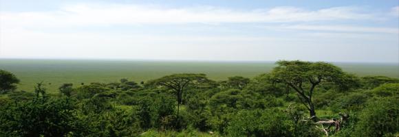
Shapefile showing the location of protected areas in Africa as national parcs and natural reserves.
Monitoring of sea surface temperature (SST) provides fundamental information on the global climate system and for the study of marine ecosystems. For example, it helps estimating heat stress conducive to coral bleaching, the process by which they expel the symbiotic algae living in their tissues and become white (bleached) and vulnerable. The NOAA Coral Reef Watch's daily global 5km satellite SST Anomaly (SSTA) compares the daily SST value with the long-term mean SST. A positive anomaly (+1.0 °C or more, warm colours) means the daily SST is warmer than the long-term average for that day; a negative anomaly (-1.0 °C or less, cold colours) means it is cooler than the average.
Ocean temperature is related to ocean heat content (the energy absorbed by the ocean), an important topic in the study of global warming. Monitoring of sea surface temperature (SST) from earth-orbiting infrared radiometers has had a wide impact on oceanographic science. It provides fundamental information on the global climate system and for the study of marine ecosystems. For example, it helps estimating heat stress conducive to coral bleaching, the process by which they expel the symbiotic algae living in their tissues and become white (bleached) and vulnerable. The NOAA Coral Reef Watch Daily Global 5km Satellite Sea Surface Temperature product (a.k.a. CoralTemp) measures the night-time ocean temperature at the sea surface, calibrated to 0.2 meters depth.
Monitoring of sea surface temperature (SST) provides fundamental information on the global climate system and for the study of marine ecosystems. For example, it helps estimating heat stress conducive to coral bleaching, the process by which they expel the symbiotic algae living in their tissues and become white (bleached) and vulnerable. The NOAA Coral Reef Watch's daily global 5km 7-day SST Trend product shows the SST trend for the most recent seven days. Pixels coloured in blue to purple follow a cooling trend while pixels coloured in yellow to red follow a warming trend. Pixels coloured in green have insignificant trends.
Forests are the most biologically diverse land ecosystems and are critical for sustaining local and global livelihoods. Deforestation can be considered a type of land degradation when forest ecosystems, with all of their important provisioning, regulating and cultural services, are exchanged for another land use, such as crop agriculture, with a narrow provisioning service focus. Damages to the land resource include the immediate reduction or loss of biomass productivity with a linked loss in habitat, biodiversity, and carbon stock. Clearance of natural forests accelerates soil erosion and the alteration of soil functioning. This layer displays the areas of concern for tree loss issues, derived from the convergence of global evidence of human-environment interactions that can have consequences on land degradation.

Africa is projected to have the fastest urban growth rate in the world — by 2050, Africa’s cities will be home to an additional 950 million people. Urban planning and management are essential development challenges. Understanding urbanisation, its drivers, dynamics and impacts, is key to designing targeted, inclusive and foward-looking policies at the local, national and continental levels. Africapolis data and evidence supports cities and governments to make urban areas more inclusive, productive and sustainable. This map of urban population covers 7 500 agglomerations in 50 countries for the base year 2015.
Water is a critical natural resource for both natural ecosystems and human subsistence. Some of the most immediate pressures on land that lead to degradation include diversion of surface waters and the removal of groundwater reserves to meet agricultural, industrial and domestic demands. This layer displays the areas of concern for water use related issues derived from the convergence of global evidence of human-environment interactions that can have consequences on land degradation. It highlights areas where the total water withdrawal (by the agriculture, industrial and domestic sectors) exceeds 40% of the total available annual renewable water supply.
This dataset provides a continent-wide, raster-based spatial representation of Earth's surface heat flow across the African tectonic plate for the year 2013, modeled under a historical baseline scenario. The data quantifies the amount of thermal energy moving from the Earth's interior to its surface, with values explicitly expressed in watts per square meter (W/m²). This resource is critical for identifying geothermal potential, understanding tectonic anomalies, and supporting broader geoscientific and energy research.
Sources and ContextThis layer is part of the Geothermal Atlas for Africa developed within the LEAP-RE project
This dataset provides the P50 projections for a geothermal system utilizing a Chiller unit.
Chiller refers to an absorption chiller or heat pump integrated into the geothermal system. It is used to provide cooling (by utilizing the geothermal heat) or to extract additional heat from the return fluid, thereby increasing the system's overall thermal harvest.
P50 is a statistical term used in risk analysis and forecasting. P50 represents the median scenario, meaning there is a 50% probability that the actual outcome will be higher than this value and a 50% probability it will be lower. It serves as the baseline "best estimate."
Metrics DefinitionsCoefficient of Performance (COP) [-]: A measure of efficiency, defined as the ratio of useful heating or cooling provided to the work (energy) required to operate the Chiller. Higher values indicate greater efficiency.
Doublet Net Production [MW]: The actual useful power output (Megawatts) generated by the "doublet" (one production well + one injection well), subtracting any energy used by pumps or auxiliary equipment.
Levelized Cost of Energy (LCOE) [US$ct/kWh]: The average revenue per unit of energy needed to recover the cost of building and operating the plant over its entire life cycle. It essentially represents the break-even price.
Net Present Value (NPV) [million US$]: The current financial value of all future cash flows the project will generate, minus the initial investment costs. A positive NPV generally indicates a profitable project.
Optimized Depth of the Aquifer [m]: The calculated ideal drilling depth (meters) to reach the geothermal reservoir that balances drilling costs with temperature/flow benefits.
Production Flow Rate [m³/h]: The volume of geothermal fluid extracted from the reservoir per hour (cubic meters per hour).
Temperature at Reservoir [°C]: The natural temperature (Celsius) of the geothermal fluid within the subsurface rock formation before it is brought to the surface.
Transmissivity [Dm]: A measure of how easily fluid flows through the porous aquifer. It is the product of hydraulic conductivity and aquifer thickness (often measured in Darcy-meters). High transmissivity means easier extraction.
Well Distance [m]: The physical distance (meters) between the production well (extraction) and the injection well (return). Proper spacing prevents "short-circuiting," where cool injected water lowers the temperature of the production well too quickly.
This dataset provides the P50 projections for a Direct Heat geothermal system.
Direct Heat refers to the use of geothermal energy for applications such as space heating, industrial processes, or agriculture. In the utilized model, it is assumed a minimum production temperature of at least 60°C and a reinjection temperature of 40°C.
P50 is a statistical term used in risk analysis and forecasting. P50 represents the median scenario, meaning there is a 50% probability that the actual outcome will be higher than this value and a 50% probability it will be lower. It serves as the baseline "best estimate."
Metrics DefinitionsCoefficient of Performance (COP) [-]: A measure of efficiency, defined as the ratio of useful heating or cooling provided to the work (energy) required to operate the Chiller. Higher values indicate greater efficiency.
Doublet Net Production [MW]: The actual useful power output (Megawatts) generated by the ""doublet"" (one production well + one injection well), subtracting any energy used by pumps or auxiliary equipment.
Levelized Cost of Energy (LCOE) [US$ct/kWh]: The average revenue per unit of energy needed to recover the cost of building and operating the plant over its entire life cycle. It essentially represents the break-even price.
Net Present Value (NPV) [million US$]: The current financial value of all future cash flows the project will generate, minus the initial investment costs. A positive NPV generally indicates a profitable project.
Optimized Depth of the Aquifer [m]: The calculated ideal drilling depth (meters) to reach the geothermal reservoir that balances drilling costs with temperature/flow benefits.
Production Flow Rate [m³/h]: The volume of geothermal fluid extracted from the reservoir per hour (cubic meters per hour).
Temperature at Reservoir [°C]: The natural temperature (Celsius) of the geothermal fluid within the subsurface rock formation before it is brought to the surface.
Transmissivity [Dm]: A measure of how easily fluid flows through the porous aquifer. It is the product of hydraulic conductivity and aquifer thickness (often measured in Darcy-meters). High transmissivity means easier extraction.
Well Distance [m]: The physical distance (meters) between the production well (extraction) and the injection well (return). Proper spacing prevents ""short-circuiting,"" where cool injected water lowers the temperature of the production well too quickly.
This dataset provides the P50 projections for a Direct Heat with Heat Pump geothermal system.
Direct Heat with Heat Pump refers to a scenario where a geothermal system is integrated with an industrial heat pump to upgrade low-grade heat. This allows for production from geothermal temperatures as low as 40°C, which are then heated by the pump to a delivery temperature of 80°C. The reinjection temperature is set to the production temperature minus 20°C, with a absolute minimum of 15°C.
P50 is a statistical term used in risk analysis and forecasting. P50 represents the median scenario, meaning there is a 50% probability that the actual outcome will be higher than this value and a 50% probability it will be lower. It serves as the baseline ""best estimate.""
Metrics DefinitionsCoefficient of Performance (COP) [-]: A measure of efficiency, defined as the ratio of useful heating or cooling provided to the work (energy) required to operate the Chiller. Higher values indicate greater efficiency.
Doublet Net Production [MW]: The actual useful power output (Megawatts) generated by the ""doublet"" (one production well + one injection well), subtracting any energy used by pumps or auxiliary equipment.
Levelized Cost of Energy (LCOE) [US$ct/kWh]: The average revenue per unit of energy needed to recover the cost of building and operating the plant over its entire life cycle. It essentially represents the break-even price.
Net Present Value (NPV) [million US$]: The current financial value of all future cash flows the project will generate, minus the initial investment costs. A positive NPV generally indicates a profitable project.
Optimized Depth of the Aquifer [m]: The calculated ideal drilling depth (meters) to reach the geothermal reservoir that balances drilling costs with temperature/flow benefits.
Production Flow Rate [m³/h]: The volume of geothermal fluid extracted from the reservoir per hour (cubic meters per hour).
Temperature at Reservoir [°C]: The natural temperature (Celsius) of the geothermal fluid within the subsurface rock formation before it is brought to the surface.
Transmissivity [Dm]: A measure of how easily fluid flows through the porous aquifer. It is the product of hydraulic conductivity and aquifer thickness (often measured in Darcy-meters). High transmissivity means easier extraction.
Well Distance [m]: The physical distance (meters) between the production well (extraction) and the injection well (return). Proper spacing prevents ""short-circuiting,"" where cool injected water lowers the temperature of the production well too quickly.
This dataset provides the P50 projections for an Organic Rankine Cycle (ORC) geothermal power plant.
Organic Rankine Cycle (ORC) refers to a binary power plant configuration where geothermal fluid (brine) is used to heat a secondary organic working fluid. This process allows for efficient electricity generation from medium-to-low temperature resources (typically 90°C to 150°C). The organic fluid vaporizes, drives a turbine, and is then condensed back into a liquid to repeat the cycle. The geothermal brine is reinjected into the reservoir after passing through the heat exchanger.
P50 is a statistical term used in risk analysis and forecasting. P50 represents the median scenario, meaning there is a 50% probability that the actual outcome will be higher than this value and a 50% probability it will be lower. It serves as the baseline ""best estimate.""
Metrics DefinitionsCoefficient of Performance (COP) [-]: A measure of efficiency, defined as the ratio of useful heating or cooling provided to the work (energy) required to operate the Chiller. Higher values indicate greater efficiency.
Doublet Net Production [MW]: The actual useful power output (Megawatts) generated by the ""doublet"" (one production well + one injection well), subtracting any energy used by pumps or auxiliary equipment.
Levelized Cost of Energy (LCOE) [US$ct/kWh]: The average revenue per unit of energy needed to recover the cost of building and operating the plant over its entire life cycle. It essentially represents the break-even price.
Net Present Value (NPV) [million US$]: The current financial value of all future cash flows the project will generate, minus the initial investment costs. A positive NPV generally indicates a profitable project.
Optimized Depth of the Aquifer [m]: The calculated ideal drilling depth (meters) to reach the geothermal reservoir that balances drilling costs with temperature/flow benefits.
Production Flow Rate [m³/h]: The volume of geothermal fluid extracted from the reservoir per hour (cubic meters per hour).
Temperature at Reservoir [°C]: The natural temperature (Celsius) of the geothermal fluid within the subsurface rock formation before it is brought to the surface.
Transmissivity [Dm]: A measure of how easily fluid flows through the porous aquifer. It is the product of hydraulic conductivity and aquifer thickness (often measured in Darcy-meters). High transmissivity means easier extraction.
Well Distance [m]: The physical distance (meters) between the production well (extraction) and the injection well (return). Proper spacing prevents ""short-circuiting,"" where cool injected water lowers the temperature of the production well too quickly.

Priority areas are identified using local coefficients estimated through Geographically Weighted Regression (GWR), which measures the spatially varying relationship between access to electricity and education using the indicator of percentage of population with secondary education .
The tool highlights locations where the local association between electricity access and the selected nutrition indicator is both negative and statistically significant. In this application, priority areas are further restricted to locations where electricity access is below 80%, ensuring that the results remain relevant for policy intervention.
The identified areas are classified as having strong, moderate, or mild associations according to the magnitude of the local GWR coefficient. This classification helps users determine the appropriate intensity of intervention. The spatially varying coefficients therefore allow users to identify areas where limited electricity access is most strongly associated with higher education, supporting targeted interventions, programme planning, and place-based development strategies.
Priority areas are identified using local coefficients estimated through Geographically Weighted Regression (GWR), which measures the spatially varying relationship between access to electricity and gender using the indicator of proportion of women with secondary school. The tool highlights locations where the local association between electricity access and the selected nutrition indicator is both negative and statistically significant. In this application, priority areas are further restricted to locations where electricity access is below 80%, ensuring that the results remain relevant for policy intervention. The identified areas are classified as having strong, moderate, or mild associations according to the magnitude of the local GWR coefficient. This classification helps users determine the appropriate intensity of intervention. The spatially varying coefficients therefore allow users to identify areas where limited electricity access is most strongly associated with lower proportion of women at secondary school, supporting targeted interventions, programme planning, and place-based development strategies.
Priority areas are identified using local coefficients estimated through Geographically Weighted Regression (GWR), which measures the spatially varying relationship between access to electricity and health using the indicator of under-5 mortality.
The tool highlights locations where the local association between electricity access and the selected nutrition indicator is both negative and statistically significant. In this application, priority areas are further restricted to locations where electricity access is below 80%, ensuring that the results remain relevant for policy intervention.
The identified areas are classified as having strong, moderate, or mild associations according to the magnitude of the local GWR coefficient. This classification helps users determine the appropriate intensity of intervention. The spatially varying coefficients therefore allow users to identify areas where limited electricity access is most strongly associated with higher mortality among children under five, supporting targeted interventions, programme planning, and place-based development strategies.

Priority areas are identified using local coefficients estimated through Geographically Weighted Regression (GWR), which measures the spatially varying relationship between access to electricity and four nutrition indicators among children under five: stunting, wasting, severe wasting, and underweight.
The tool highlights locations where the local association between electricity access and the selected nutrition indicator is both negative and statistically significant. In this application, priority areas are further restricted to locations where electricity access is below 80%, ensuring that the results remain relevant for policy intervention.
The identified areas are classified as having strong, moderate, or mild associations according to the magnitude of the local GWR coefficient. This classification helps users determine the appropriate intensity of intervention. The spatially varying coefficients therefore allow users to identify areas where limited electricity access is most strongly associated with poorer nutritional outcomes among children under five, supporting targeted interventions, programme planning, and place-based development strategies.
Priority areas are identified using local coefficients estimated through Geographically Weighted Regression (GWR), which measures the spatially varying relationship between access to sanitation infrastructure and education using the indicator of percentage of population with secondary education . The tool highlights locations where the local association between electricity access and the selected nutrition indicator is both negative and statistically significant. The identified areas are classified as having strong, moderate, or mild associations according to the magnitude of the local GWR coefficient. This classification helps users determine the appropriate intensity of intervention. The spatially varying coefficients therefore allow users to identify areas where limited sanitation access is most strongly associated with lower education, supporting targeted interventions, programme planning, and place-based development strategies.
Priority areas are identified using local coefficients estimated through Geographically Weighted Regression (GWR), which measures the spatially varying relationship between access to sanitation infrastructure and gender using the indicator of percentage of women with secondary education. The tool highlights locations where the local association between sanitation access and the selected gender indicator is both negative and statistically significant. The identified areas are classified as having strong, moderate, or mild associations according to the magnitude of the local GWR coefficient. This classification helps users determine the appropriate intensity of intervention. The spatially varying coefficients therefore allow users to identify areas where limited sanitation access is most strongly associated with lower women education, supporting targeted interventions, programme planning, and place-based development strategies.

Priority areas are identified using local coefficients estimated through Geographically Weighted Regression (GWR), which measures the spatially varying relationship between access to sanitation and four nutrition indicators among children under five: stunting, wasting, severe wasting, and underweight.
The tool highlights locations where the local association between sanitation access and the selected nutrition indicator is both negative and statistically significant. In this application, priority areas are further restricted to locations where sanitation access is below 80%, ensuring that the results remain relevant for policy intervention.
The identified areas are classified as having strong, moderate, or mild associations according to the magnitude of the local GWR coefficient. This classification helps users determine the appropriate intensity of intervention. The spatially varying coefficients therefore allow users to identify areas where limited sanitation access is most strongly associated with poorer child nutrition outcomes, supporting targeted interventions, programme planning and place-based development strategies.

This dataset represents a geographic clip to Africa of the World Database on Protected Areas (WDPA), which is the authoritative and most complete global dataset on terrestrial and marine protected areas. The parent database is a joint initiative between the UN Environment Programme (UNEP) and the International Union for Conservation of Nature (IUCN), managed by the UNEP World Conservation Monitoring Centre (UNEP-WCMC). Information is submitted and verified by international secretariats, national and regional governments, NGOs, communities, and landowners.
This spatial dataset has been specifically filtered and clipped to include only protected areas located within the terrestrial and marine boundaries of the African continent and its associated island nations.
The dataset comprises both spatial data (GIS boundaries) and attribute data (descriptive information) for protected sites across Africa. Key attributes include site name, designation type (national, regional, or international), governance model, IUCN management category, marine/terrestrial status, and legal establishment date.
The WDPA is the primary global mechanism used to track progress toward international area-based conservation targets. This African subset is widely used across various sectors for:
The global WDPA dataset is updated and released on a monthly basis through the Protected Planet platform. This clip was extracted on May 2026.