Food crisis response planning can save lives if put in place in a timely manner. To do this, decision makers must be warned of climate extreme events impacting agricultural production. The Anomaly hotSpot of Agricultural Production tool (ASAP) is an online decision support system for early warning about hotspots of agricultural production anomaly (crop and rangeland), developed by the JRC for food security crises prevention and response planning anticipation. This map shows the frequency at which countries were classified as hotspots for agricultural production problems between 2004 and 2018. Hotspots are identified on a monthly basis.

Food crisis response planning can save lives if put in place in a timely manner. To do this, decision makers must be warned of climate extreme events impacting agricultural production. The Anomaly hotSpot of Agricultural Production tool (ASAP) is an online decision support system for early warning about hotspots of agricultural production anomaly (crop and rangeland), developed by the JRC for food security crises prevention and response planning anticipation. This map shows the frequency of ASAP anomaly warnings for crop growth for 2004-2018. It highlights the high sensitivity of the main agricultural areas in Northern Africa, the Horn of Africa and the Southern African Development Community to drought conditions.

Food crisis response planning can save lives if put in place in a timely manner. To do this, decision makers must be warned of climate extreme events impacting agricultural production. The Anomaly hotSpot of Agricultural Production tool (ASAP) is an online decision support system for early warning about hotspots of agricultural production anomaly (crop and rangeland), developed by the JRC for food security crises prevention and response planning anticipation. This map shows the frequency of ASAP anomaly warnings for rangeland growth for 2004-2018. It highlights the high sensitivity of the main agricultural areas in Northern Africa, the Horn of Africa and the Southern African Development Community to drought conditions.

This dataset provides the P50 projections for a geothermal system utilizing a Chiller unit.

Chiller refers to an absorption chiller or heat pump integrated into the geothermal system. It is used to provide cooling (by utilizing the geothermal heat) or to extract additional heat from the return fluid, thereby increasing the system's overall thermal harvest.

P50 is a statistical term used in risk analysis and forecasting. P50 represents the median scenario, meaning there is a 50% probability that the actual outcome will be higher than this value and a 50% probability it will be lower. It serves as the baseline "best estimate."

• Coefficient of Performance (COP) [-]: A measure of efficiency, defined as the ratio of useful heating or cooling provided to the work (energy) required to operate the Chiller. Higher values indicate greater efficiency.

• Doublet Net Production [MW]: The actual useful power output (Megawatts) generated by the "doublet" (one production well + one injection well), subtracting any energy used by pumps or auxiliary equipment.

• Levelized Cost of Energy (LCOE) [US$ct/kWh]: The average revenue per unit of energy needed to recover the cost of building and operating the plant over its entire life cycle. It essentially represents the break-even price.

• Net Present Value (NPV) [million US$]: The current financial value of all future cash flows the project will generate, minus the initial investment costs. A positive NPV generally indicates a profitable project.

• Optimized Depth of the Aquifer [m]: The calculated ideal drilling depth (meters) to reach the geothermal reservoir that balances drilling costs with temperature/flow benefits.

• Pressure needed to drive pumps [Bar]: The total pressure difference required to drive the thermal loop through the reservoir and wellbore.

• Production Flow Rate [m³/h]: The volume of geothermal fluid extracted from the reservoir per hour (cubic meters per hour).

• Temperature at Reservoir [°C]: The natural temperature (Celsius) of the geothermal fluid within the subsurface rock formation before it is brought to the surface.

• Transmissivity [Dm]: A measure of how easily fluid flows through the porous aquifer. It is the product of hydraulic conductivity and aquifer thickness (often measured in Darcy-meters). High transmissivity means easier extraction.

• Well Distance [m]: The physical distance (meters) between the production well (extraction) and the injection well (return). Proper spacing prevents "short-circuiting," where cool injected water lowers the temperature of the production well too quickly.

This dataset provides the P50 projections for a Direct Heat geothermal system.

Direct Heat refers to the use of geothermal energy for applications such as space heating, industrial processes, or agriculture. In the utilized model, it is assumed a minimum production temperature of at least 60°C and a reinjection temperature of 40°C.

P50 is a statistical term used in risk analysis and forecasting. P50 represents the median scenario, meaning there is a 50% probability that the actual outcome will be higher than this value and a 50% probability it will be lower. It serves as the baseline "best estimate."

• Coefficient of Performance (COP) [-]: A measure of efficiency, defined as the ratio of useful heating or cooling provided to the work (energy) required to operate the Chiller. Higher values indicate greater efficiency.

• Doublet Net Production [MW]: The actual useful power output (Megawatts) generated by the ""doublet"" (one production well + one injection well), subtracting any energy used by pumps or auxiliary equipment.

• Levelized Cost of Energy (LCOE) [US$ct/kWh]: The average revenue per unit of energy needed to recover the cost of building and operating the plant over its entire life cycle. It essentially represents the break-even price.

• Net Present Value (NPV) [million US$]: The current financial value of all future cash flows the project will generate, minus the initial investment costs. A positive NPV generally indicates a profitable project.

• Optimized Depth of the Aquifer [m]: The calculated ideal drilling depth (meters) to reach the geothermal reservoir that balances drilling costs with temperature/flow benefits.

• Pressure needed to drive pumps [Bar]: The total pressure difference required to drive the thermal loop through the reservoir and wellbore.

• Production Flow Rate [m³/h]: The volume of geothermal fluid extracted from the reservoir per hour (cubic meters per hour).

• Temperature at Reservoir [°C]: The natural temperature (Celsius) of the geothermal fluid within the subsurface rock formation before it is brought to the surface.

• Transmissivity [Dm]: A measure of how easily fluid flows through the porous aquifer. It is the product of hydraulic conductivity and aquifer thickness (often measured in Darcy-meters). High transmissivity means easier extraction.

• Well Distance [m]: The physical distance (meters) between the production well (extraction) and the injection well (return). Proper spacing prevents ""short-circuiting,"" where cool injected water lowers the temperature of the production well too quickly.

This dataset provides the P50 projections for a Direct Heat with Heat Pump geothermal system.

Direct Heat with Heat Pump refers to a scenario where a geothermal system is integrated with an industrial heat pump to upgrade low-grade heat. This allows for production from geothermal temperatures as low as 40°C, which are then heated by the pump to a delivery temperature of 80°C. The reinjection temperature is set to the production temperature minus 20°C, with a absolute minimum of 15°C.

P50 is a statistical term used in risk analysis and forecasting. P50 represents the median scenario, meaning there is a 50% probability that the actual outcome will be higher than this value and a 50% probability it will be lower. It serves as the baseline ""best estimate.""

• Coefficient of Performance (COP) [-]: A measure of efficiency, defined as the ratio of useful heating or cooling provided to the work (energy) required to operate the Chiller. Higher values indicate greater efficiency.

• Doublet Net Production [MW]: The actual useful power output (Megawatts) generated by the ""doublet"" (one production well + one injection well), subtracting any energy used by pumps or auxiliary equipment.

• Levelized Cost of Energy (LCOE) [US$ct/kWh]: The average revenue per unit of energy needed to recover the cost of building and operating the plant over its entire life cycle. It essentially represents the break-even price.

• Net Present Value (NPV) [million US$]: The current financial value of all future cash flows the project will generate, minus the initial investment costs. A positive NPV generally indicates a profitable project.

• Optimized Depth of the Aquifer [m]: The calculated ideal drilling depth (meters) to reach the geothermal reservoir that balances drilling costs with temperature/flow benefits.

• Pressure needed to drive pumps [Bar]: The total pressure difference required to drive the thermal loop through the reservoir and wellbore.

• Production Flow Rate [m³/h]: The volume of geothermal fluid extracted from the reservoir per hour (cubic meters per hour).

• Temperature at Reservoir [°C]: The natural temperature (Celsius) of the geothermal fluid within the subsurface rock formation before it is brought to the surface.

• Transmissivity [Dm]: A measure of how easily fluid flows through the porous aquifer. It is the product of hydraulic conductivity and aquifer thickness (often measured in Darcy-meters). High transmissivity means easier extraction.

• Well Distance [m]: The physical distance (meters) between the production well (extraction) and the injection well (return). Proper spacing prevents ""short-circuiting,"" where cool injected water lowers the temperature of the production well too quickly.

This dataset provides the P50 projections for an Organic Rankine Cycle (ORC) geothermal power plant.

Organic Rankine Cycle (ORC) refers to a binary power plant configuration where geothermal fluid (brine) is used to heat a secondary organic working fluid. This process allows for efficient electricity generation from medium-to-low temperature resources (typically 90°C to 150°C). The organic fluid vaporizes, drives a turbine, and is then condensed back into a liquid to repeat the cycle. The geothermal brine is reinjected into the reservoir after passing through the heat exchanger.

P50 is a statistical term used in risk analysis and forecasting. P50 represents the median scenario, meaning there is a 50% probability that the actual outcome will be higher than this value and a 50% probability it will be lower. It serves as the baseline ""best estimate.""

• Coefficient of Performance (COP) [-]: A measure of efficiency, defined as the ratio of useful heating or cooling provided to the work (energy) required to operate the Chiller. Higher values indicate greater efficiency.

• Doublet Net Production [MW]: The actual useful power output (Megawatts) generated by the ""doublet"" (one production well + one injection well), subtracting any energy used by pumps or auxiliary equipment.

• Levelized Cost of Energy (LCOE) [US$ct/kWh]: The average revenue per unit of energy needed to recover the cost of building and operating the plant over its entire life cycle. It essentially represents the break-even price.

• Net Present Value (NPV) [million US$]: The current financial value of all future cash flows the project will generate, minus the initial investment costs. A positive NPV generally indicates a profitable project.

• Optimized Depth of the Aquifer [m]: The calculated ideal drilling depth (meters) to reach the geothermal reservoir that balances drilling costs with temperature/flow benefits.

• Pressure needed to drive pumps [Bar]: The total pressure difference required to drive the thermal loop through the reservoir and wellbore.

• Production Flow Rate [m³/h]: The volume of geothermal fluid extracted from the reservoir per hour (cubic meters per hour).

• Temperature at Reservoir [°C]: The natural temperature (Celsius) of the geothermal fluid within the subsurface rock formation before it is brought to the surface.

• Transmissivity [Dm]: A measure of how easily fluid flows through the porous aquifer. It is the product of hydraulic conductivity and aquifer thickness (often measured in Darcy-meters). High transmissivity means easier extraction.

• Well Distance [m]: The physical distance (meters) between the production well (extraction) and the injection well (return). Proper spacing prevents ""short-circuiting,"" where cool injected water lowers the temperature of the production well too quickly.

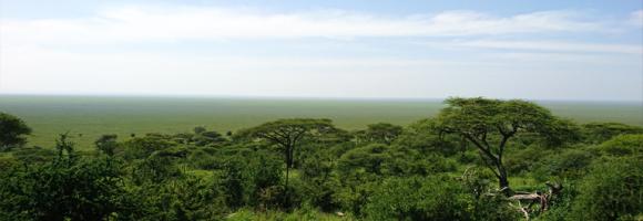
Biodiversity hotspots are the Earth’s most biologically rich—yet heavily threatened—terrestrial regions. These are regions where success in conserving species can have an enormous impact in securing our global biodiversity. To qualify as a biodiversity hotspot, an area must meet two strict criteria: it must contain at least 1,500 species of vascular plants found nowhere else on Earth (known as "endemic" species), and it must have lost at least 70% of its primary native vegetation. 36 regions are identified as hotspots by Conservation International and partners, 9 of which lay (partially or fully) in Africa. This dataset shows their location.

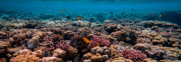
Healthy coral reefs provide a home for millions of aquatic species. They protect coastal homes from storms and support commercial and subsistence fisheries as well as jobs and businesses through tourism and recreation. Yet they are severely threatened by pollution, disease, habitat destruction and climate change. When corals are stressed, they expel the symbiotic algae living in their tissues and become white (bleached) and vulnerable. Corals are vulnerable to bleaching when the sea surface temperature (SST) exceeds the temperatures normally experienced in the hottest month of the year. The NOAA Coral Reef Watch daily global 5km Coral Bleaching HotSpot product measures the occurrence and magnitude of instantaneous heat stress, potentially resulting in coral bleaching. It highlights regions where the SST is warmer than the highest monthly mean. HotSpot values of 1°C or more indicate heat stress leading to coral bleaching and are highlighted in yellow to dark red colors.

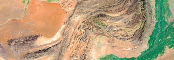
Humans need increasingly more biomass for food, fodder, fibre and energy. Meeting these demands changes global ecosystems. Tracking changes in total biomass production or land productivity is an essential part of monitoring land transformations that are typically associated with land degradation. Land productivity dynamics (LPD) are used as an indicator of change or stability of the land’s capacity to sustain primary production. This layer displays the areas of concern for land productivity related issues, derived from the convergence of global evidence of human-environment interactions that can have consequences on land degradation.

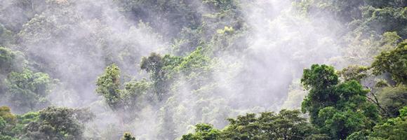
This layer presents the Effective Leaf Area Index (LAIe) Anomalies, representing the deviation of current vegetation density from the historical average. Monitoring the change of LAI is essential for assessing the evolution of the vegetation over Africa.

LAI anomalies are calculated relative to the average values between 2003 and 2010. The dataset captures LAI anomalies every 10 days, reflecting the high variability and rapid changes in African vegetation cover. Increases in temperature and precipitation deficits are the primary drivers for negative anomalies (reduced foliage density). Beyond climatic factors, human activities or animal grazing may also locally impact the state and density of leaves.

This layer is part of the a href="https://fapar.jrc.ec.europa.eu/_www/index.php">Earth Land Information System (ELIS).

The Fraction of Photosynthetically Active Radiation Absorbed (FAPAR) is used to track the overall primary productivity associated with atmospheric CO2 fixation. FAPAR anomalies relative to the average between 2003 and 2010 show large surface variations, in terms of values and coverage, of vegetation productivity conditions over Africa. Temperature and precipitation deficits are the main drivers for the negative anomalies. Each location with a negative anomaly (FAPAR value lower than the long-term mean for that location – shades of red) indicates relative vegetation stress during that 10-day interval. Each location with a positive anomaly (FAPAR value higher than long-term mean for that location – shades of green) indicates relative favourable vegetation growth conditions during that 10-day interval. FAPAR values and their anomalies provide useful information for water and agricultural management purposes.

This layer is part of the Earth Land Information System (ELIS).

The application of fertiliser is a key component in increasing agricultural production. However, there are thresholds beyond which the cost of inputs fails to lead to corresponding increases in yield. Beyond economic inefficiency, overuse of commercial inorganic fertiliser can also result in a decline in soil condition and structure, including reduced soil carbon content, water-holding capacity and porosity, and to environmental pollution. This layer displays the areas of concern for high-input agriculture related issues derived from the convergence of global evidence of human-environment interactions that can have land degradation consequences.

This layer is part of the World Altas of Desertification

Many African countries, especially in the Sub-Saharan region highly depend on hydropower which is one of the energy sources that are most affected by droughts. At the same time hydropower has a huge impact on water consumption (mainly through evaporation from reservoir surfaces) in comparison with other fuel types despite having higher densities of plants and installed capacities. Hydropower accounts for 15% of Africa’s energy production. This map shows the energy production (GWh) of hydropower plants with an installed capacity above 5MW, aggregated for each hydropower-generating country in Africa for year 2016.

The hydropower installed capacity indicates the amount of energy a hydropower plant can produce in its turbines. In 2016, hydropower accounted for 54% of the installed capacity in Eastern Africa, 58% in Central Africa and 30% in Western Africa with fourteen countries having a hydropower share above 50% and eight countries above 70%. These highly hydropower-dependent countries are particularly prone to electricity cuts due to the lack of water caused by severe droughts. This map shows the location and installed capacities of hydropower plants above 5MW installed capacity in Africa for year 2016, representing 95% of the total hydropower installed capacity in Africa.

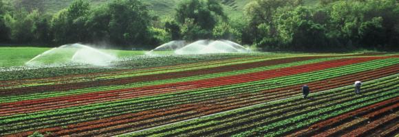
Humans need increasingly more biomass for food, fodder, fiber and energy. In Africa, circa 22% of the vegetated land surface showed a decline or unstable land productivity between 1999 and 2013. Persistent reduction of land productivity points to long-term alteration of the health and productive capacity of the land, which are characteristic of land degradation. It has impact on ecosystem services and benefits, thus on the sustainable livelihoods of human communities. This map shows the dynamics of (vegetated) land productivity over a time period, in other terms the trajectories of above-ground biomass. It reflects changes in ecosystem functioning e.g. vegetation growth cycles due to natural variation and/or human intervention, and can be associated with processes of land degradation or recovery. The 5 classes depict two levels of persistent productivity decline, one level of instability or stress in capacity, one level of stable productivity and one level of increased productivity.

Smallholder farmers have limited access to capital and are reluctant to trade their low-risk system (low input and low yield) to a high-risk system (high input and potentially higher yields). But Insufficient application of fertilizer on agricultural land may lead to soil nutrients depletion, lower yields, and eventually land abandonment. This layer displays the areas of concern for low-input agriculture related issues derived from the convergence of global evidence of human-environment interactions that can have land degradation consequences.

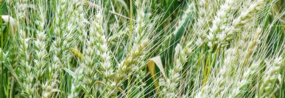
The map is based on Copernicus Global Land Cover data which shows actual land cover (what physically covers land across the globe—forests, grasslands, croplands, lakes, wetlands, built-up area, etc) at 100m x 100m resolution. The land cover data for Africa was overlaid on (high resolution) satellite imagery of Africa, which is then used to determine the land use (by visual interpretation) associated with the various land cover patterns on the Copernicus Global Land Cover map.

Copernicus land cover data offers several advantages: it is of high quality, has a high resolution (100m x 100m), and offers time series satellite imagery. More importantly, the Copernicus Global Land Service is a continuous process and its datasets are updated annually. This means that the Soils4Africa map of agricultural land can be updated every time the land cover data for the new year becomes available (the map is currently based on 2019 data).

The Copernicus dataset already includes the category ‘cropland,’ which by definition is part of agricultural land. The Soils4Africa map broadens the scope of that dataset by infering information on agricultural use and including other kinds of agricultural land use such as grazing pastures and plantations.

When land is mapped as other than ‘cropland'-- like ‘shrubland’ for example-- it is more difficult to interpret and determine whether it is under agricultural use. The Copernicus dataset includes information about ‘fractional cover’-- or the percentage of a particular pixel under a particular kind of land cover (for example, 30% of a 100m x 100m pixel could be forest and 20% could be shrubland). The Soils4Africa map takes into account how fractional cover varies over an area to establish rules for interpreting its land cover data to determine whether it is under agricultural use and for what purpose. These rules were validated by comparing it with ground level information on land use (or land use pattern) for specific areas drawn from the interpretation of satellite imagery from Google Earth.

For example, ground-level observation shows that forest cover upwards of 30% in a given area when matched by shrubland cover of over 30%, is characterized by woody vegetation with a smooth canopy. Therefore, such area is more likely to be under plantations rather than natural forest. Thus, such an area should be counted as agricultural land, even if less than 15% of it is under crops.

Monitoring of sea surface temperature (SST) provides fundamental information on the global climate system and for the study of marine ecosystems. This layer compares the SST value of the last full month with the long-term mean SST. A positive anomaly (warm colours) means the monthly SST is warmer than the long-term average for that month; a negative anomaly (cool colours) means it is cooler than the average.

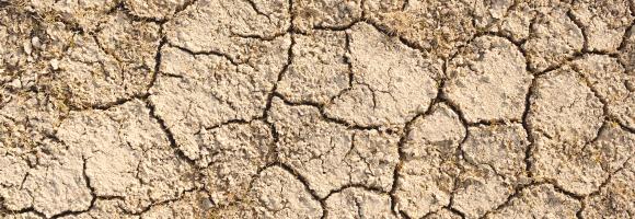
Droughts affect millions of people in the world each year and have long-lasting socioeconomic impacts. They can occur over most parts of the world, even in wet and humid regions, and can profoundly impact agriculture, basic household welfare, tourism, ecosystems and the services they provide. The Risk of Drought Impact for Agriculture (RDrI-Agri) is a categorized risk index, indicating the probability of having impacts from a drought, with particular focus on vegetation. Higher risk (in red) means that the areas affected will be the most likely to report impacts due to droughts. It is updated every ten days.

Monitoring of sea surface temperature (SST) provides fundamental information on the global climate system and for the study of marine ecosystems. For example, it helps estimating heat stress conducive to coral bleaching, the process by which they expel the symbiotic algae living in their tissues and become white (bleached) and vulnerable. The NOAA Coral Reef Watch's daily global 5km satellite SST Anomaly (SSTA) compares the daily SST value with the long-term mean SST. A positive anomaly (+1.0 °C or more, warm colours) means the daily SST is warmer than the long-term average for that day; a negative anomaly (-1.0 °C or less, cold colours) means it is cooler than the average.

Agricultural drought events can affect large regions across the world. Soil moisture (or soil water content) is an important variable for plant growth, and - together with precipitation and evapotranspiration - is a basic component of the hydrological cycle. The Soil Moisture Anomaly (SMA) indicator is used to detect and monitor agricultural drought, that is when there is reduced crop production due to insufficient soil moisture. It is computed as a deviation from the climatological reference period, and is updated 3 times a month (after the 10th, the 20th and the last day of the month). This layer displays the map for the last full decade of the current month. Negative anomalies (shades of brown) represent dry conditions.

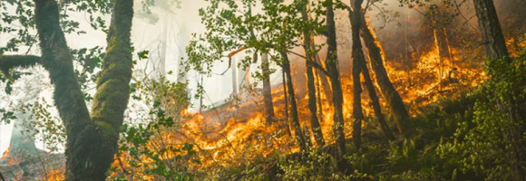
Vegetation fires have become a major concern in Africa because of their negative impacts on the environment and on human welfare. Uncontrolled (and un-prescribed) wildfires cause forest and vegetation degradation and related biodiversity loss, resulting in immediate and long-term impacts on the livelihoods of local communities and upstream impacts on national and regional economies. Fires in the tropical environment are a major contributor to tropical forest degradation and, if too frequent, can lead to savannisation of these areas. Vegetation fires are also a significant source of trace gases and aerosols in the atmosphere and contribute to the anticipated climate change, particularly with emissions of CO2. This layer shows the deviation of dekadal fire occurrences from the long-term average of the same 10-day period. A positive anomaly means more fire events than average for the last full 10-day period (red). A negative anomaly means less fire events than average for the last full 10-day period (green).

Chlorophyll-a concentrations (Chla) are an indicator of phytoplankton abundance and biomass in open waters. They can be an effective measure of trophic status and are commonly used to measure water quality. This layer compares the Chla value from the last full month with the long-term mean Chla. A positive anomaly (warm colours) means the monthly Chla is higher than the long-term average for that month; a negative anomaly (cool colours) means it is lower than the average.

Increasing water scarcity and water quality issues are serious constraints in Africa and worldwide. Measuring precipitation anomalies is important for detecting and characterizing meteorological droughts, and, in the agricultural sector especially, for effectively managing climate related uncertainties. This layer shows the deviation of the precipitations of the last full month from the long-term average of the same month. A positive anomaly (shades of blue) means there was more rainfall than average during that month. A negative anomaly (yellow to red) means there was less rainfall than average during that month.